Data Analysis
Andrey Shestakov (avshestakov@hse.ru)
Clustering 2: Quality and Mixture models1
1. Some materials are taken from machine learning course of Victor Kitov
Cluster Validity and Quality Measures
General approaches
- Evaluate using "ground-truth" clustering (Quality Measure)
- invariant to cluster naming
- Unsupervised criterion (Cluster Validity)
- based on intuition:
- objects from same cluster should be similar
- objects from different clusters should be different
- based on intuition:
Based on ground-truth
Rand Index
$$ \text{Rand}(\hat{\pi},\pi^*) = \frac{a + d}{a + b + c + d} \text{,}$$ where
- $a$ - number of pairs that are grouped both in $\hat{\pi}$ and $\pi^*$
$d$ - number of pairs that are separated both in $\hat{\pi}$ and $\pi^*$
$b$ ($c$) - number of pairs that are separated both in $\hat{\pi}$ ($\pi^*$), but grouped in $\pi^*$ ($\hat{\pi}$)
Rand Index
$$ \text{Rand}(\hat{\pi},\pi^*) = \frac{tp + tn}{tp + fp + fn + tn} \text{,}$$ where
- $tp$ - number of pairs that are grouped both in $\hat{\pi}$ and $\pi^*$,
$tn$ - number of pairs that are separated both in $\hat{\pi}$ and $\pi^*$
$fp$ ($fn$) - number of pairs that are separated both in $\hat{\pi}$ ($\pi^*$), but grouped in $\pi^*$ ($\hat{\pi}$)
Adjusted Rand Index
$$\text{ARI}(\hat{\pi},\pi^*) = \frac{\text{Rand}(\hat{\pi},\pi^*) - \text{Expected}}{\text{Max} - \text{Expected}}$$
Check wikipedia =)
Precision, Recall, F-measure
- $\text{Precision}(\hat{\pi},\pi^*) = \frac{tp}{tp+fn}$
- $\text{Recall}(\hat{\pi},\pi^*) = \frac{tp}{tp+fp}$
- $\text{F-measure}(\hat{\pi},\pi^*) = \frac{2\cdot Precision \cdot Recall}{Precision + Recall}$
Cluster validity
- Intuition
- objects from same cluster should be similar
- objects from different clusters should be different
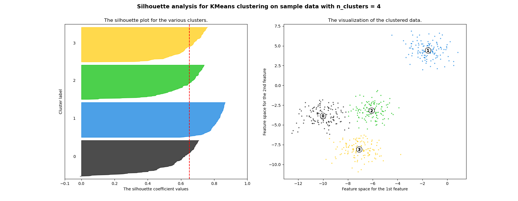
Silhouette
For each object $x_{i}$ define:
- $s_{i}$-mean distance to objects in the same cluster
- $d_{i}$-mean distance to objects in the next nearest cluster Silhouette coefficient for $x_{i}$: $$ Silhouette_{i}=\frac{d_{i}-s_{i}}{\max\{d_{i},s_{i}\}} $$
Silhouette coefficient for $x_{1},...x_{N}$: $$ Silhouette=\frac{1}{N}\sum_{i=1}^{N}\frac{d_{i}-s_{i}}{\max\{d_{i},s_{i}\}} $$
Discussion
Advantages
- The score is bounded between -1 for incorrect clustering and +1 for highly dense clustering.
- Scores around zero indicate overlapping clusters.
- The score is higher when clusters are dense and well separated.
Disadvantages
- complexity $O(N^{2}D)$
- favours convex clusters
Mixture models
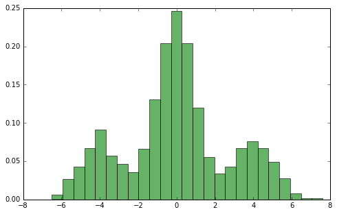
Sample density
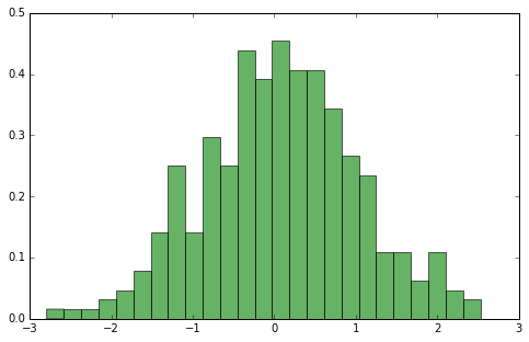
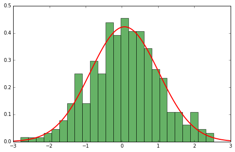
Parametric density approximation
It can be accurately modelled with existing parametric family - Normal
$$ p(x | \theta) = \mathcal{N}(x|\mu, \sigma) = \frac{1}{\sqrt{2\pi\sigma^2}}\exp\left({-\frac{(x-\mu)^2}{2\sigma^2}}\right) $$ or shall we.. $$ p(x | \theta) = \mathcal{N}(x|\mu, \Sigma) = \frac{1}{(2\pi\Sigma)^{1/2}}\exp\left(-\frac{1}{2}(x-\mu)^\top\Sigma^{-1}(x-\mu)\right) $$
 </cetner>
ML Method for estimating parameters
- Consider (log of) likelihood
$$ \begin{align} L(x) = & \prod\limits_{i=1}^B\mathcal{N}(x_i|\mu, \Sigma)\rightarrow \max\limits_{\mu, \Sigma} \end{align} $$
- Take derivatives and equate them to zero
$$\mu_{ML} = \frac 1 N \sum_{i=1}^N x_i, \quad \mathbf{\Sigma}_{ML} = \frac 1 N \sum_{i=1}^N (x_i - \mu_{ML}) (x_i - \mu_{ML})^T$$
 </cetner>
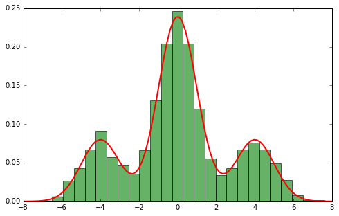
Mixture models
$$ p(x)=\sum_{z=1}^{Z}\phi_{z}p(x|\theta_{z}) $$
- $Z$ - number of components
- $\phi_{z},\,z=1,2,...Z$ - mixture component probabilities, $\phi_{z}\ge0,\,\sum_{z=1}^{Z}\phi_{z}=1$
- $p(x|\theta_{z})$ - component density functions
- Parameters of mixture model $\Theta=\{\phi_{z},\theta_{z},\,z=1,2,...Z\}$
$p(x|\theta_{z})$ may be of single or different parametric families.
Mixture of Gaussians
Gaussians model continious r.v. on $(-\infty,+\infty)$.
$$p(x|\theta_{z})=N(x|\mu_{z},\Sigma_{z}),\,\theta_{z}=\{\mu_{z},\Sigma_{z}\}$$
$$ p(x)=\sum_{z=1}^{Z}\phi_{z}N(x|\mu_{z},\Sigma_{z}) $$
Problems
- Again consider (log of) likelihood
$$ \begin{align} L(x) = & \sum_{i=1}^N \log p(x_i) = \sum_{i=1}^N\log\left(\sum_{z=1}^{Z}\phi_{z}N(x|\mu_{z},\Sigma_{z})\right) \rightarrow \max\limits_{\mu_z, \Sigma_z, \phi_z} \end{align} $$
- No closed form solution..
- Use EM-algorithm!
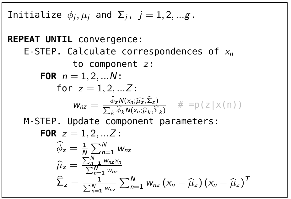
Expectation-Maximization
- Let's say we know (fixed) all $\mu_k$-s, $\Sigma_k$-s and $\phi_k$-s.
- Introduce posteriour probabilty of object $x_i$ belonging to component $z$: $$ w_{iz} = p(z | x) = \frac{p(z) p(x_i | z)}{\sum_{k=1}^K p(k) p(x_i | k)} = \frac{\phi_z \mathcal{N}(x_i | \mu_z, \Sigma_z)}{\sum_{k=1}^K \phi_k \mathcal{N}(x_i | \mu_k, \Sigma_k)} $$
$$ \sum_k w_{ik} = 1 $$
- Now with given soft assignments re-estimate the parameters: $$ \phi_k = \frac{ \sum_{i=1}^N w_{ik} }{N}, \;\; \mu_k = \frac{\sum_{i=1}^N w_{ik} x_i}{\sum_{i=1}^N w_{ik}} $$ $$ \Sigma_k = \frac {\sum_{i=1}^N w_{ik} (x_i - \mu_k)^\top (x_i - \mu_k)}{\sum_{i=1}^N w_{ik}} $$
Expectation-Maximization
- Does that somehow correspont to k-means algorithm?
EM illustration
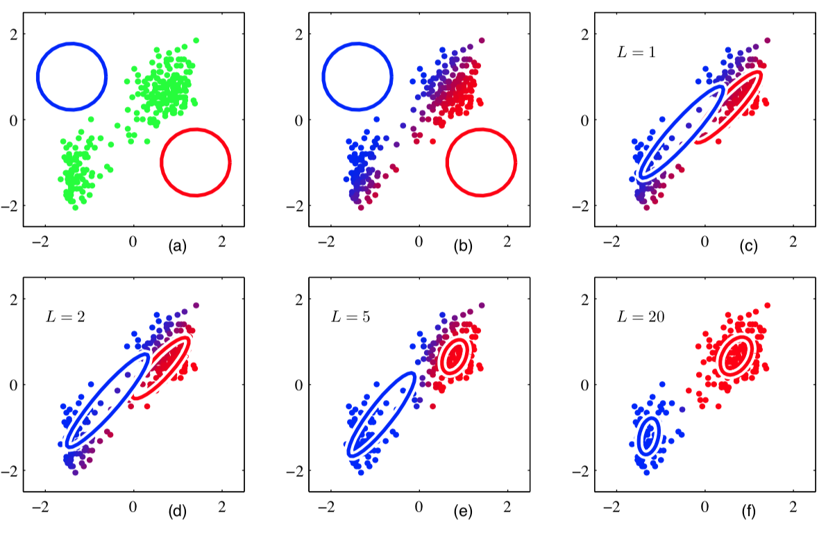
K-means versus EM clustering
- For each $x_{i}$ EM algorithm gives $w_{iz}=p(z|x_{i})$.
- This is soft or probabilistic clustering into $Z$ clusters, having priors $\phi_{1},...\phi_{Z}$ and probability distributions $p(x;\theta_{1}),...p(x;\theta_{Z})$.
We can make it hard clustering using $z_{i}=\arg\max_{z}w_{iz}$.
EM clustering becomes K-means clustering when:
- applied to Gaussians
- with equal priors
- with unity covariance matrices
- with hard clustering
Initialization for Gaussian mixture EM
- Fit K-means to $x_{1},x_{2},...x_{N}$, obtain cluster centers $\mu_{z},\,z=1,2,...Z$ and cluster assignments $z_{1},z_{2},...z_{N}$. \item Initialize mixture probabilities $$ \widehat{\phi}_{z}\propto\sum_{i=1}^{N}\mathbb{I}[z_{i}=z] $$
- Initialize Gaussian means with cluster centers $\mu_{z},\,z=1,2,...Z$.
- Initialize Gaussian covariance matrices with $$ \widehat{\Sigma}_{z}=\frac{1}{\sum_{i=1}^{N}\mathbb{I}[z_{i}=z]}\sum_{n=1}^{N}\mathbb{I}[z_{i}=z]\left(x_{i}-\mu_{z}\right)\left(x_{i}-\mu_{z}\right)^{T} $$
Properties of EM
- Many local optima exist
- in particular likelihood$\to\infty$ when $\mu_{z}=x_{i}$ and $\sigma_{z}\to0$
- Only local optimum is found with EM
- Results depends on initialization
- It is common to run algorithm multiple times with different initializations and then select the result maximizing the likelihood function.
- Number of components may be selected with:
- cross-validation on the final task
- out-of-sample maximum likelihood
Simplifications of Gaussian mixtures
Simplifications of Gaussian mixtures
- $\Sigma_{z}\in\mathbb{R}^{DxD}$ requires $\frac{D(D+1)}{2}$ parameters.
- Covariance matrices for $Z$ components require $Z\frac{D(D+1)}{2}$ parameters.
- Components can be poorly identified when
- $Z\frac{D(D+1)}{2}$ is large compared to $N$
- when components are not well separated
- In these cases we can impose restrictions on covariance matrices.
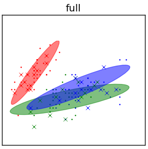
Unrestricted covariance matrices
- full covariance matrices $\Sigma_{z},\,z=1,2,...Z$.
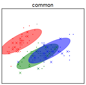
Common covariance matrix
- $\Sigma_{1}=\Sigma_{2}=...=\Sigma_{Z}$
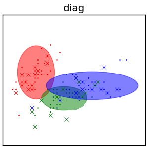
Diagonal covariance matrices
- $\Sigma_{z}=\text{diag}\{\sigma_{z,1}^{2},\sigma_{z,2}^{2}...\sigma_{z,D}^{2}\}$
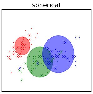
Spherical matrices
- $\Sigma_{z}=\sigma_{z}^{2}I$, $I\in\mathbb{R}^{DxD}$ - identity matrix