Data Analysis

Andrey Shestakov (avshestakov@hse.ru)

Neural Networks 1¹

^{1. Some materials are taken from machine learning course of Victor Kitov}

Let's recall previous lecture¶

Boosting, Ensembles¶

Construction of multiple models to increase model quality
- In parallel (Bagging, Blending, Stacking, Random Forest)
- Sequentially (Boosting)
Works great!
Hard to interpret
Tricky parameter tuning

Neural Networks¶

History¶

Neural networks originally appeared as an attempt to model human brain
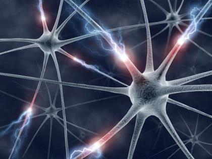
Human brain consists of multiple interconnected neuron cells
- cerebral cortex (the largest part) is estimated to contain 15-33 billion neurons
- communication is performed by sending electrical and electro-chemical signals
- signals are transmitted through axons - long thin parts of neurons.

History ¶

1943 – The first mathematical model of a neural network (Walter Pitts and Warren McCulloch)
1957 – Setting the foundation for deep neural networks (Frank Rosenblatt)
1965 – The first working deep learning networks
1979-80 – An ANN learns how to recognize visual patterns
1982 – The creation of the Hopfield Networks
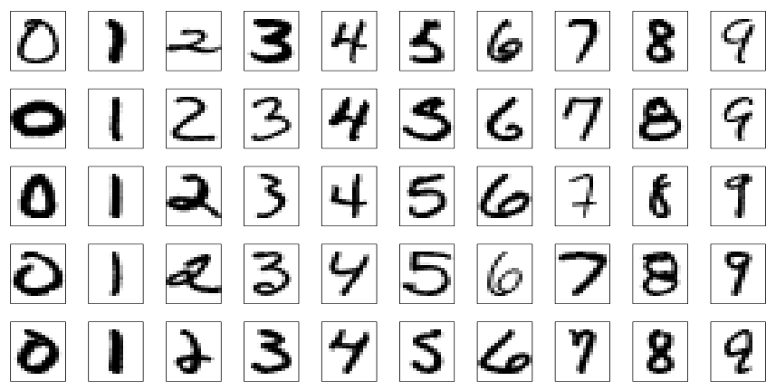
1989 – Machines read handwritten digits (Yann LeCun)
1997 – Long short-term memory was proposed (Jürgen Schmidhuber and Sepp Hochreiter)
1998 – Gradient-based learning (Yann LeCun)
2011 – Creation of AlexNet
2014 – Generative Adversarial Networks (GAN)

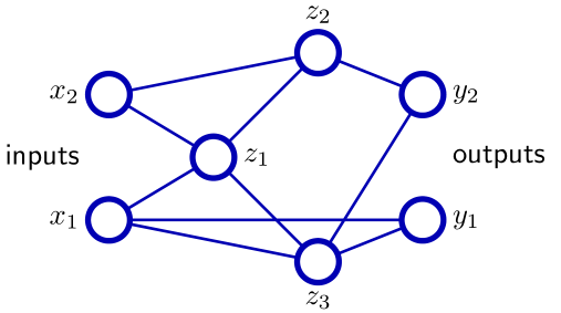
Simple model of a neuron¶

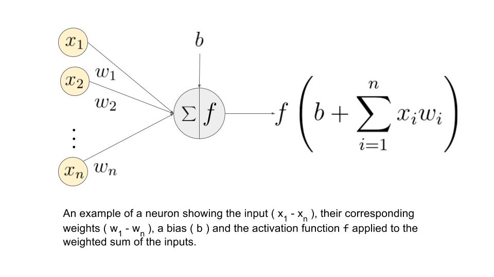
Neuron get's activated in the half-space, defined by $w_{0}+w_{1}x^{1}+w_{2}x^{2}+...+w_{D}x^{D}\ge0$.
Each node is called a neuron
Each edge is associated a weight
Constant feature $b$ stands for bias

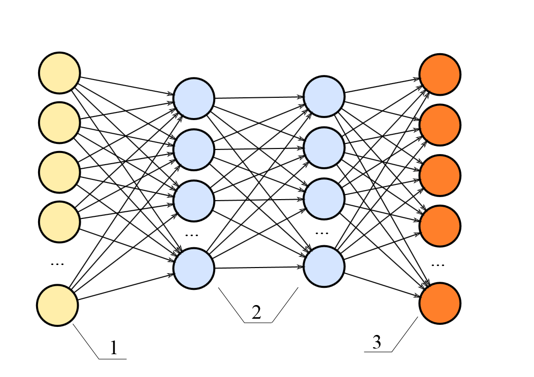
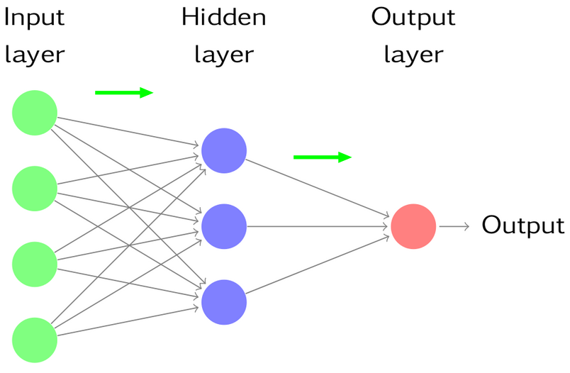
Multilayer perceptron architecture¶

Hierarchically nested set of neurons.
Each node has its own weights.

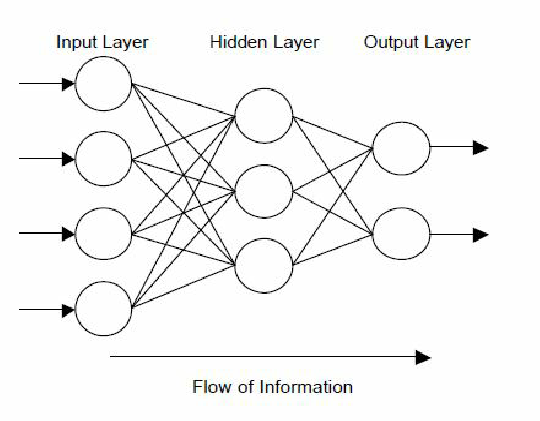
This is structure of multilayer perceptron - acyclic directed graph.

Layers¶

Structure of neural network:
- 1-input layer
- 2-hidden layers
- 3-output layer

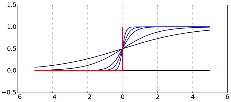
Continious activations¶

Pitfall of $\mathbb{I}[]$: it causes stepwise constant outputs, weight optimization methods become inapliccable.
We can replace $\mathbb{I}[w^{T}x+w_{0}\ge0]$ with smooth activation $f(w^{T}x+w_{0})$

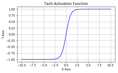
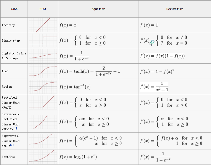
Typical activation functions¶

sigmoidal: $\sigma(x)=\frac{1}{1+e^{-x}}$
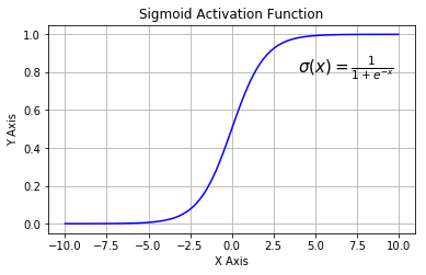
- 1-layer neural network with sigmoidal activation is equivalent to logistic regression
hyperbolic tangent: $tangh(x)=\frac{e^{x}-e^{-x}}{e^{x}+e^{-x}}$

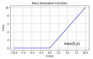
Typical activation functions¶

ReLU: $f(x)=[x]_{+}$.

Activation function zoo¶

Definition details¶

Label each neuron with integer $j$.
Denote: $I_{j}$ - input to neuron $j$, $O_{j}$ - output of neuron $j$
Input to neuron $j$: $I_{j}=\sum_{k\in inc(j)}w_{kj}O_{k}+w_{0j}$,
Output of neuron $j$: $O_{j}=f(I_{j})$.
- $w_{0j}$ is the bias term
- $f(x)$ is the activation function
- $inc(j)$ is a set of neurons with outgoing edges incoming to neuron $j$.
- further we will assume that at each layer there is a vertex with constant output $O_{const}\equiv1$, so we can simplify notation

$$ I_{j}=\sum_{k\in inc(j)}w_{kj}O_{k} $$

Output Generation¶

Output generation¶

Forward propagation is a process of successive calculations of neuron outputs for given features.

Activations at output layer¶

Regression: $f(I)=I$ (linear activation)
Classification:
- binary: $y\in\{+1,-1\}$ $$ f(I)=p(y=+1|x)=\frac{1}{1+e^{-I}} $$
- multiclass: $y\in{1,2,...C}$ $$ f(I_{1},...I_{C})=p(y=j|x)=\frac{e^{I_{j}}}{\sum_{k=1}^{C}e^{I_{k}}},\,j=1,2,...C $$ where $I_{1},...I_{C}$ are inputs of output layer.

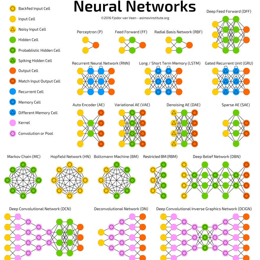
Generalizations¶

each neuron $j$ may have custom non-linear transformation $f_{j}$
weights may be constrained:
- non-negative
- equal weights
- etc.
layer skips are possible
Not considered here: RBF-networks, recurrent networks.

Number of layers selection¶

Number of layers usually denotes all layers except input layer (hidden layers+output layer)
Classification:
- single layer network selects arbitrary half-spaces
- 2-layer network selects arbitrary convex polyhedron (by intersection of 1-layer outputs)
  - therefore it can approximate arbitrary convex sets
- 3-layer network selects (by union of 2-layer outputs) arbitrary finite sets of polyhedra
  - therefore it can approximate almost all sets with well defined volume

Number of layers selection¶

Regression:
- single layer can approximate arbitrary linear function
- 2-layer network can model indicator function of arbitrary convex polyhedron
- 3-layer network can uniformly approximate arbitrary continuous function (as sum weighted sum of indicators convex polyhedra)

Sufficient amount of layers

Any continuous function on a compact space can be uniformly approximated by 2-layer neural network with linear output and wide range of activation functions (excluding polynomial).

In practice often it is more convenient to use more layers with less total amount of neurons
- model becomes more interpretable and easy to fit.

TensorFlow PlayGround ¶

Neural network optimization¶

Network optimization: regression¶

Single output:

$$ \frac{1}{N}\sum_{n=1}^{N}(\widehat{y}_{n}(x_{n})-y_{n})^{2}\to\min_{w} $$

K outputs

$$ \frac{1}{NK}\sum_{n=1}^{N}\sum_{k=1}^{K}(\widehat{y}_{nk}(x_{n})-y_{nk})^{2}\to\min_{w} $$

Network optimization: classification¶

Two classes ($y\in\{0,1\}$, $p=P(y=1)$): $$ \prod_{n=1}^{N}p(y_{n}=1|x_{n})^{y_{n}}[1-p(y_{n}=1|x_{n})]{}^{1-y_{n}}\to\max_{w} $$
$C$ classes ($y_{nc}=\mathbb{I}\{y_{n}=c\}$):

$$ \prod_{n=1}^{N}\prod_{c=1}^{C}p(y_{n}=c|x_{n})^{y_{nc}}\to\max_{w} $$

In practice log-likelihood (cross-entropy) is maximized

Neural network optimization¶

Let $L(\widehat{y},y)$ denote the loss function of output

We may optimize neural network using gradient descent:

k=0 initialize randomly w_0 # small values for sigmoid and tangh

while stop criteria not met:
```
  w_k+1 := w_k - alpha * grad(L(w_k))
  k := k+1
```
Standardization of features makes gradient descend converge faster

Gradient calculation¶

Let $W$ denote the total dimensionality of weights space
Direct $\nabla E(w)$ calculation, using $$ \frac{\partial L}{\partial w_{i}}=\frac{L(w+\varepsilon_{i})-L(w)}{\varepsilon}+O(\varepsilon)\label{eq:deriv1} $$ or better $$ \frac{\partial L}{\partial w_{i}}=\frac{L(w+\varepsilon_{i})-L(w-\varepsilon_{i})}{2\varepsilon}+O(\varepsilon^{2})\label{eq:deriv2} $$ has complexity: $O(W^{2})$
- need to calculate $W$ derivatives
- complexity for each derivative: $2W$

Backpropagation algorithm needs only $O(W)$ to evaluate all derivatives.

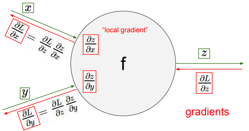
Backpropagation algorithm¶

Idea¶

Definitions¶

Denote $w_{ij}$ be the weight of edge, connecting $i$-th and $j$-th neuron
Define $\delta_j = \frac{\partial L}{\partial I_j} = \frac{\partial L}{\partial O_j}\frac{\partial O_j}{\partial I_j}$
Since $L$ depends on $w_{ij}$ through the following functional relationship $L(w_{ij}) = L\left(O_j\left(I_j(w_{ij})\right)\right)$, using the chain rule we get: $$ \frac{\partial L}{\partial w_{ij}} = \frac{\partial L}{\partial I_j}\frac{\partial I_j}{\partial w_{ij}} = \delta_j O_i$$ because $\frac{\partial I_j}{\partial w_{ij}} = \frac{\partial}{\partial w_{ij}} \left(\sum\limits_{k\in inc(j)} w_{kj} O_k\right) = O_i$, where $inc(j)$ is a set of neurons with outgoing edges to neuron $j$
$\frac{\partial L}{\partial I_j} = \frac{\partial L}{\partial O_j}\frac{\partial O_j}{\partial I_j} = \frac{\partial L}{\partial O_j} f'(I_j) $

Output layer¶

If neuron $j$ belongs to the output node, then error $\frac{\partial L}{\partial O_j}$ is calculated directly
For output layer $\delta_j$ are calculated directly: $$ \delta_j= \frac{\partial L}{\partial O_j}\frac{\partial O_j}{\partial I_j} = \frac{\partial L}{\partial O_j} f'(I_j) \qquad (1)$$
Example (single point $x$ and true vector of outputs $(y_1,\dots,y_{|OL|})$:
- For $L = \frac{1}{2}\sum\limits_{j\in OL}(O_j - y_j)^2$ $$ \frac{\partial L}{\partial O_j} = O_j - y_j $$
- Sigmoid activation function: $$ f'(I_j) = \sigma(I_j)(1-\sigma(I_j)) = O_j(1-O_j) $$
- finally $$ \delta_j = (O_j - y_j)O_j(1-O_j)$$

Inner layer¶

If neuron $j$ belongs to some hidden layer, denote $out(j) = \{k_1, k_2, \dots, k_m\}$ the set of all neurons, receiving output of neuron $j$ as their input
The effect of $O_j$ on $L$ in fully absorbed by $I_{k_1},I_{k_2},\dots,I_{k_m}$, so $$ \frac{\partial L(O_j)}{\partial O_j} = \frac{\delta L(I_{k_1},I_{k_2},\dots,I_{k_m})}{\delta O_j} = \sum\limits_{k\in out(j)} \left( \frac{\partial L}{\partial I_k} \frac{\partial I_k}{\partial O_j} \right) = \sum\limits_{k\in out(j)} \left(\delta_k w_{jk}\right)$$
So for layers other than output layer we have: $$ \delta_j = \frac{\partial L}{\partial I_j} = \frac{\partial L}{\partial O_j}\frac{\partial O_j}{\partial I_j} = \sum\limits_{k\in out(j)} \left(\delta_k w_{jk}\right) f'(I_j) \qquad (2)$$
Weight derivatives are calculated useing errors and outputs: $$ \frac{\partial L}{\partial w_{ij}} = \frac{\partial L}{\partial I_j}\frac{\partial I_j}{\partial w_{ij}} = \delta_jO_j \qquad (3)$$

Backprop¶

Forward propagate $x_n$ to the neural network, store all inputs $I_j$ and outputs $O_j$ for each neuron
Calculate $\delta_i$ for all $i \in$ output layer using $(1)$
Propagate $\delta_i$ from final layer back layer by layer $(2)$
Using calculated deltas and outputs calculate $\frac{\partial L}{\partial w_{ij}}$ with $(3)$

Options:
- batch
- (min-batch) stochastic

Multiple local optima problem¶

Optimization problem for neural nets is \textbf{non-convex}.
Different optima will correspond to:
- different starting parameter values
- different training samples
So we may solve task many times for different conditions and then
- select best model
- alternatively: average different obtained models to get ensemble
And/Or use some complex optimization methods

Vanishing Gradient Problem¶

In [3]:

x = np.linspace(-10, 10, 1000)
gr_sigm = sigmoid(x)*(1-sigmoid(x))

plt.plot(x, gr_sigm)

Out[3]:

[<matplotlib.lines.Line2D at 0x116792f90>]

Feature scaling
Careful weight initialization
Using ReLU activation function

Model complexity and overfitting¶

Constrain model directly:
- constrain number of neurons
- constrain number of layes
- impose constraints on weights
Take a flexible model
- early stopping (with validation set)
- L2 regularization $$ L(w) + \lambda\sum_i w_i^2 $$
Augmentation (more used in convnets)

Case study: ZIP codes recognition¶

ZIP code recognition task

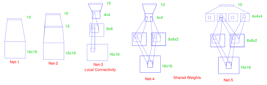
Neural network structures¶

Net1: no hidden layer
Net2: 1 hidden layer, 12 hidden units fully connected
Net3: 2 hidden layers, locally connected
Net4: 2 hidden layers, locally connected with weight sharing
Net5: 2 hidden layers, locally connected, 2 levels of weight sharing

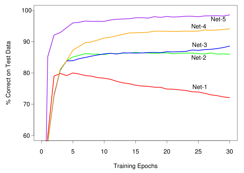
Results¶

Conclusion¶

Advantages of neural networks:
- can model accurately complex non-linear relationships
- easily parallelizable
Disadvantages of neural networks:
- hardly interpretable ("black-box" algorithm)
- optimization requires skill
  - too many parameters
  - may converge slowly
  - may converge to inefficient local minimum far from global one

Data Analysis

Andrey Shestakov (avshestakov@hse.ru)

Neural Networks 11

Let's recall previous lecture¶

Boosting, Ensembles¶

Neural Networks¶

History¶

History¶

Simple model of a neuron¶

Multilayer perceptron architecture¶

Layers¶

Continious activations¶

Typical activation functions¶

Typical activation functions¶

Activation function zoo¶

Definition details¶

Output Generation¶

Output generation¶

Activations at output layer¶

Generalizations¶

Number of layers selection¶

Number of layers selection¶

TensorFlow PlayGround¶

Neural network optimization¶

Network optimization: regression¶

Network optimization: classification¶

Neural network optimization¶

Gradient calculation¶

Backpropagation algorithm¶

Idea¶

Definitions¶

Output layer¶

Inner layer¶

Backprop¶

Multiple local optima problem¶

Vanishing Gradient Problem¶

Model complexity and overfitting¶

Case study: ZIP codes recognition¶

Neural network structures¶

Results¶

Conclusion¶

Useful Refs¶

Neural Networks 1¹

History ¶

TensorFlow PlayGround ¶