Data Analysis
Andrey Shestakov (avshestakov@hse.ru)
Boosting.1
1. Some materials are taken from machine learning course of Victor Kitov
Boosting
Linear ensembles
$$ F(x)=f_{0}(x)+\alpha_{1}h_{1}(x)+...+\alpha_{M}h_{M}(x) $$Regression: $\widehat{y}(x)=F(x)$
Binary classification: $score(y|x)=F(x),\,\widehat{y}(x)= sign(F(x))$
- Notation: $h_{1}(x),...h_{M}(x)$ are called base learners, weak learners, base models.
- Too expensive to optimize $f_{0}(x),h_{1}(x),...h_{M}(x)$ and $\alpha_{1},...\alpha_{M}$ jointly for large $M$.
- May lead to overfitting
- Idea: optimize $f_{0}(x)$ and then each pair $(h_{m}(x),\,\alpha_{m})$ greedily.
Forward stagewise additive modeling (FSAM)
Input:
- training dataset $(x_{i},y_{i}),\,i=1,2,...N$;
- loss function $\mathcal{L}(f,y)$,
- general form of "base learner" $h(x|\gamma)$ (dependent from parameter $\gamma$)
- number $M$ of successive additive approximations.
ALGORITHM:
- Fit initial approximation $f_{0}(x)=\arg\min_{f}\sum_{i=1}^{N}\mathcal{L}(f(x_{i}),y_{i})$
For $m=1,2,...M$:
- find next best classifier $$ (\alpha_{m},h_{m})=\arg\min_{h,c}\sum_{i=1}^{N}\mathcal{L}(f_{m-1}(x_{i})+\alpha h(x_{i}),\,y_{i}) $$
- set $$ f_{m}(x)=f_{m-1}(x)+\alpha_{m}h_{m}(x) $$ Output: approximation function $f_{M}(x)=f_{0}(x)+\sum_{m=1}^{M}\alpha_{m}h_{m}(x)$
Comments on FSAM
- Number of steps $M$ should be determined by performance on validation set.
- Step 1 need not be solved accurately, since its mistakes are expected to be corrected by future base learners.
- we can take $f_{0}(x)=\arg\min_{\beta\in\mathbb{R}}\sum_{i=1}^{N}\mathcal{L}(\beta,y_{i})$ or simply $f_{0}(x)\equiv0$.
- By similar reasoning there is no need to solve 2.A accurately
- typically very simple base learners are used such as trees of depth=1,2,3.
- For some loss functions, such as $\mathcal{L}(y,f(x))=e^{-yf(x)}$ we can solve FSAM explicitly.
- For general loss functions gradient boosting scheme should be used.
AdaBoost
Adaboost (discrete version): assumptions
- binary classification task $y\in\{+1,-1\}$
- family of base classifiers $h(x)=h(x|\gamma)$ where $\gamma$ is some fixed parametrization.
- $h(x)\in\{+1,-1\}$
- classification is performed with $\widehat{y}=sign\{f_{0}(x)+\alpha_{1}f_{1}(x)+...+\alpha_{M}f_{M}(x)\}$
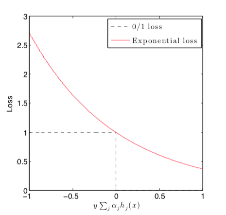
- optimized loss is $\mathcal{L}(y,f(x))=e^{-yf(x)}$
- FSAM is applied
Exponential loss
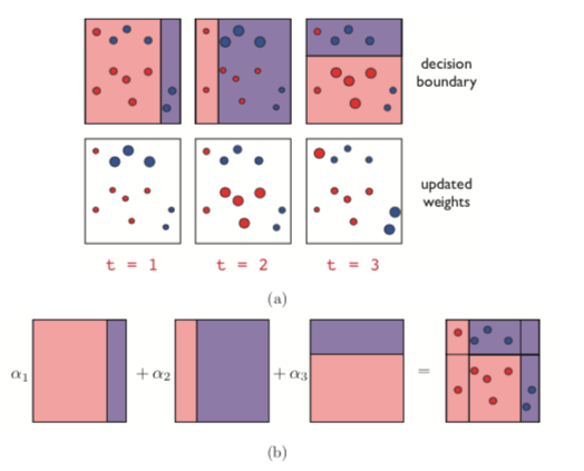
Adaboost (discrete version): algorithm
Input: training dataset $(x_{i},y_{i}),\,i=1,2,...n$; number of additive weak classifiers $M$, a family of weak classifiers $h(x)\in\{+1,-1\}$, trainable on weighted datasets.
ALGORITHM:
- Initialize observation weights $w_{i}=1/n$, $i=1,2,...n$.
for $m=1,2,...M$:
- fit $h^{m}(x)$ to training data using weights $w_{i}$
- compute weighted misclassification rate: $$ E_{m}=\sum_{i=1}^{N}w_{i}\mathbb{I}[h^{m}(x_i)\ne y_{i}] $$
- compute $\alpha_{m}=\frac{1}{2}\ln\left((1-E_{m})/E_{m}\right)$
- update sample weights: $$ w_{i}\leftarrow \frac{w_{i}e^{-\alpha_{m}y_i h^{m}(x_i)}}{W},$$ Where $W$ is normalization factor $\left(W = \sum_i w_i e^{-\alpha_m y_i h^m(x_i)}\right)$
Output: composite classifier $f(x)=sign\left(\sum_{m=1}^{M}\alpha_{m}h^{m}(x)\right)$
X = np.array([[-2, -1], [-2, 1], [2, -1], [2, 1], [-1, -1], [-1, 1], [1, -1], [1, 1]])
y = np.array([-1,-1,-1,-1,1,1,1,1])

plt.scatter(X[:, 0], X[:, 1], c=y, s=500)

ada = AdaBoostClassifier(n_estimators=3, algorithm='SAMME',
                         base_estimator=DecisionTreeClassifier(max_depth=1))
ada.fit(X, y)

plot_decision(ada)
ada.estimator_weights_

X, y = make_moons(noise=0.1)
plt.figure(figsize=(17,15))
plt.scatter(X[:, 0], X[:, 1], c=y)

interact(ada_demo, n_est=IntSlider(min=1, max=150, value=1, step=1))
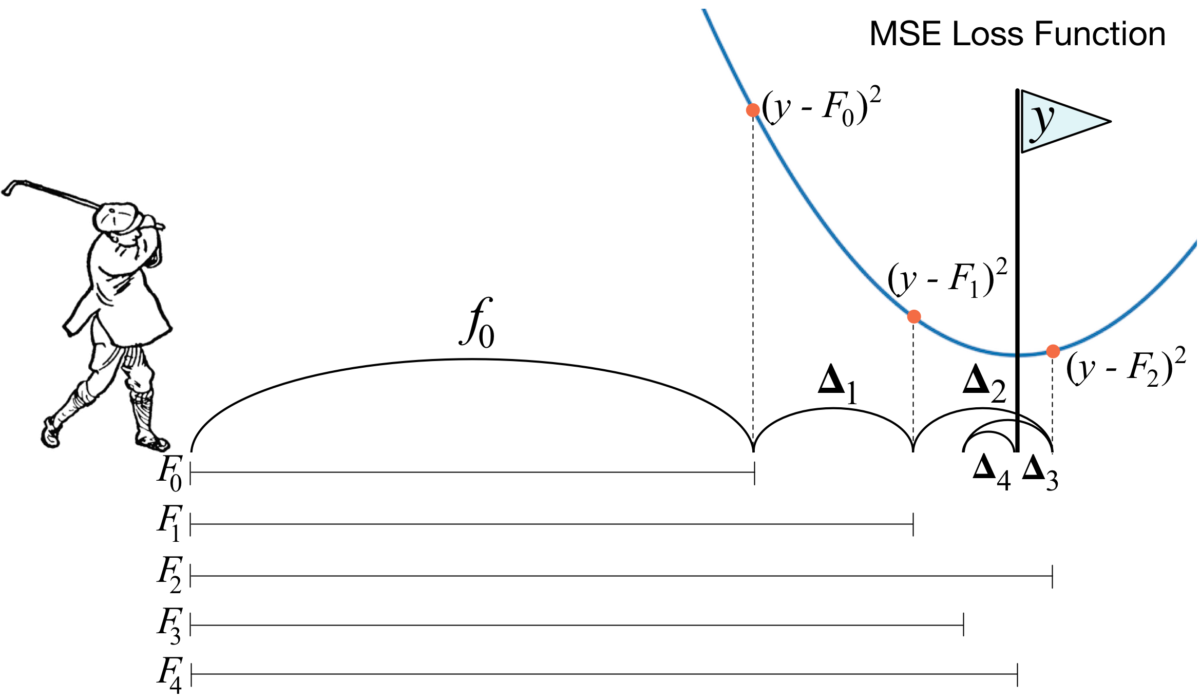
Gradient boosting
Motivation
- Problem: For general loss function $L$ FSAM cannot be solved explicitly
- Analogy with function minimization: when we can't find optimum explicitly we use numerical methods
- Gradient boosting: numerical method for iterative loss minimization
Gradient descent algorithm
$$ F(w)\to\min_{w},\quad w\in\mathbb{R}^{N} $$Gradient descend algorithm:
Input: $\eta$-parameter, controlling the speed of convergence $M$-number of iterations
ALGORITHM:
- initialize $w$
- for $m=1,2,...M$:
- $\Delta w = \frac{\partial F(w)}{\partial w}$
- $w = w-\eta \Delta w$
Gradient boosting
- Now consider $F\left(f(x_{1}),...f(x_{N})\right)=\sum_{n=1}^{N}\mathcal{L}\left(f(x_{n}),y_{n}\right)$
- Gradient descent performs pointwise optimization, but we need generalization, so we optimize in space of functions.
- Gradient boosting implements modified gradient descent in function space:
- find $z_{i}=-\frac{\partial\mathcal{L}(r,y_{i})}{\partial r}|_{r=f^{m-1}(x_{i})}$
- fit base learner $h_{m}(x)$ to $\left\{ (x_{i},z_{i})\right\} _{i=1}^{N}$

interact(grad_small_demo,
         n_est=IntSlider(min=0, max=50, value=0, step=1),
         learning_rate=FloatSlider(min=0.1, max=1., value=0.1, step=0.05),
         max_depth=IntSlider(min=1, max=5, value=1, step=1))
Gradient boosting
Input: training dataset $(x_{i},y_{i}),\,i=1,2,...N$; loss function $\mathcal{L}(f,y)$; learning rate $\nu$ and the number $M$ of successive additive approximations.
- Fit initial approximation $f_{0}(x)$ (might be taken $f_{0}(x)\equiv0$)
For each step $m=1,2,...M$:
- calculate derivatives $z_{i}=-\frac{\partial\mathcal{L}(r,y_{i})}{\partial r}|_{r=f^{m-1}(x_{i})}$
- fit $h_{m}$ to $\{(x_{i},z_{i})\}_{i=1}^{N}$, for example by solving $$ \sum_{n=1}^{N}(h_{m}(x_{n})-z_{n})^{2}\to\min_{h_{m}} $$
- set $f_{m}(x)=f_{m-1}(x)+\nu h_{m}(x)$
Output: approximation function $f_{M}(x)=f_{0}(x)+\sum_{m=1}^{M}\nu h_{m}(x)$
- What changes with classification?
- Nothing!

y = np.array([0, 0, 1, 1, 0])
X = np.array([
    [1,1],
    [2,1],
    [1,2],
    [-1,1],
    [-1,0],
])

plt.scatter(X[:, 0], X[:, 1], c=y, cmap='flag')

interact(grad_small_demo_class,
         n_est=IntSlider(min=1, max=50, value=1, step=1),
         learning_rate=FloatSlider(min=0.1, max=1., value=0.1, step=0.05),
         max_depth=IntSlider(min=1, max=5, value=1, step=1))
interact(grad_demo, n_est=IntSlider(min=1, max=150, value=1, step=1))
Modified gradient descent algorithm
Input: $M$-number of iterations
ALGORITHM:
- initialize $w$
- for $m=1,2,...M$:
- $\Delta w = \frac{\partial F(w)}{\partial w}$
- $c^* = \arg\min_c F(w-c \Delta w)$
- $w = w-c^* \Delta w$
Gradient boosting with optimal coefficient
Input: training dataset $(x_{i},y_{i}),\,i=1,2,...N$; loss function $\mathcal{L}(f,y)$; learning rate $\nu$ and the number $M$ of successive additive approximations.
- Fit initial approximation $f_{0}(x)$ (might be taken $f_{0}(x)\equiv0$)
For each step $m=1,2,...M$:
- calculate derivatives $z_{i}=-\frac{\partial\mathcal{L}(r,y_{i})}{\partial r}|_{r=f^{m-1}(x_{i})}$
- fit $h_{m}$ to $\{(x_{i},z_{i})\}_{i=1}^{N}$, for example by solving $$ \sum_{n=1}^{N}(h_{m}(x_{n})-z_{n})^{2}\to\min_{h_{m}} $$
solve univariate optimization problem: $$ \sum_{i=1}^{N}\mathcal{L}\left(f_{m-1}(x_{i})+c_{m}h_{m}(x_{i}),y_{i}\right)\to\min_{c_{m}\in\mathbb{R}_{+}} $$
set $f_{m}(x)=f_{m-1}(x)+c_m h_{m}(x)$
Output: approximation function $f_{M}(x)=f_{0}(x)+\sum_{m=1}^{M}c_m h_{m}(x)$
Gradient boosting of trees
Input : training dataset $(x_{i},y_{i}),\,i=1,2,...N$; loss function $\mathcal{L}(f,y)$ and the number $M$ of successive additive approximations.
- Fit constant initial approximation $f_{0}(x)$: $f_{0}(x)=\arg\min_{\gamma}\sum_{i=1}^{N}\mathcal{L}(\gamma,\,y_{i})$
- For each step $m=1,2,...M$:
- calculate derivatives $z_{i}=-\frac{\partial\mathcal{L}(r,y)}{\partial r}|_{r=f^{m-1}(x)}$
- fit regression tree $h^{m}$ on $\{(x_{i},z_{i})\}_{i=1}^{N}$ with some loss function, get leaf regions $\{R_{j}^{m}\}_{j=1}^{J_{m}}$.
- for each terminal region $R_{j}^{m}$, $j=1,2,...J_{m}$ solve univariate optimization problem: $$ \gamma_{j}^{m}=\arg\min_{\gamma}\sum_{x_{i}\in R_{j}^{m}}\mathcal{L}(f_{m-1}(x_{i})+\gamma,\,y_{i}) $$
- update $f_{m}(x)=f_{m-1}(x)+\sum_{j=1}^{J_{m}}\gamma_{j}^{m}\mathbb{I}[x\in R_{j}^{m}]$
Output: approximation function $f_{M}(x)$
Modification of boosting for trees
- Compared to first method of gradient boosting, boosting of regression trees finds additive coefficients individually for each terminal region $R_{j}^{m}$, not globally for the whole classifier $h^{m}(x)$.
- This is done to increase accuracy: forward stagewise algorithm cannot be applied to find $R_{j}^{m}$, but it can be applied to find $\gamma_{j}^{m}$, because second task is solvable for arbitrary $L$.
- Max leaves $J$
- interaction between no more than $J-1$ terms
- $M$ controls underfitting-overfitting tradeoff and selected using validation set
Shrinkage & subsampling
- Shrinkage of general GB, step (d): $$ f_{m}(x)=f_{m-1}(x)+\nu c_{m}h_{m}(x) $$
- Shrinkage of trees GB, step (d):
Comments:
- $\nu\in(0,1]$
- $\nu \text{ decreases } \implies M \text{ increases } $
Subsampling
- increases speed of fitting
- may increase accuracy
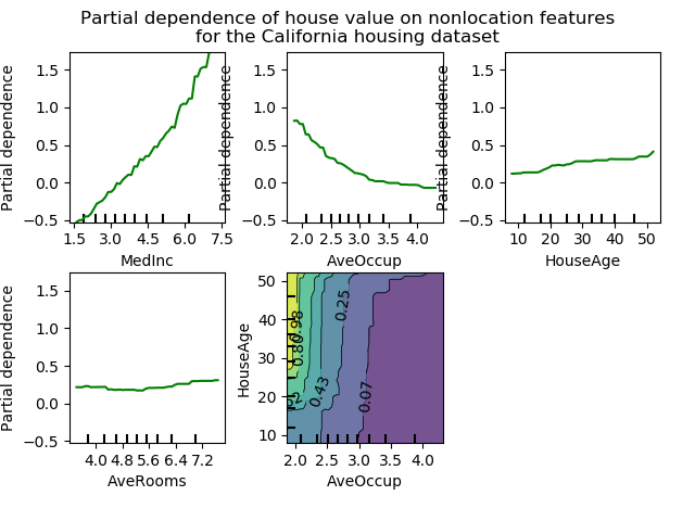
Interpretation - partial dependency plots
- Problem - we have huge black-box model $\hat{y}^k = F(x^k_1, x^k_2,\dots,x^k_p)$
- Want to have at least some interpretation
- Idea - cosider a single predictor $x_j$
- Find out its influence on prediction after we have "averaged out" the influence of all other variables: