Data Analysis
Andrey Shestakov (avshestakov@hse.ru)
Metric-based models1
Nearest Centroid, K-NN
1. Some materials are taken from machine learning course of Victor Kitov
Let's recall previous lecture
- Machine learning algorithms reconstruct relationship between features $x$ and outputs $y$.
- Design matrix $X=[\mathbf{x}_{1},...\mathbf{x}_{M}]^{T}$, $Y=[y_{1},...y_{M}]^{T}$.
- Relationship is reconstructed by optimal function $\widehat{y}=f_{\widehat{\theta}}(x)$ from function class $\{f_{\theta}(x),\,\theta\in\Theta\}$.
- Empirical risk appriximation
- Hold-out validation
- Cross-validation
- A/B testing
Overfitting - Underfitting
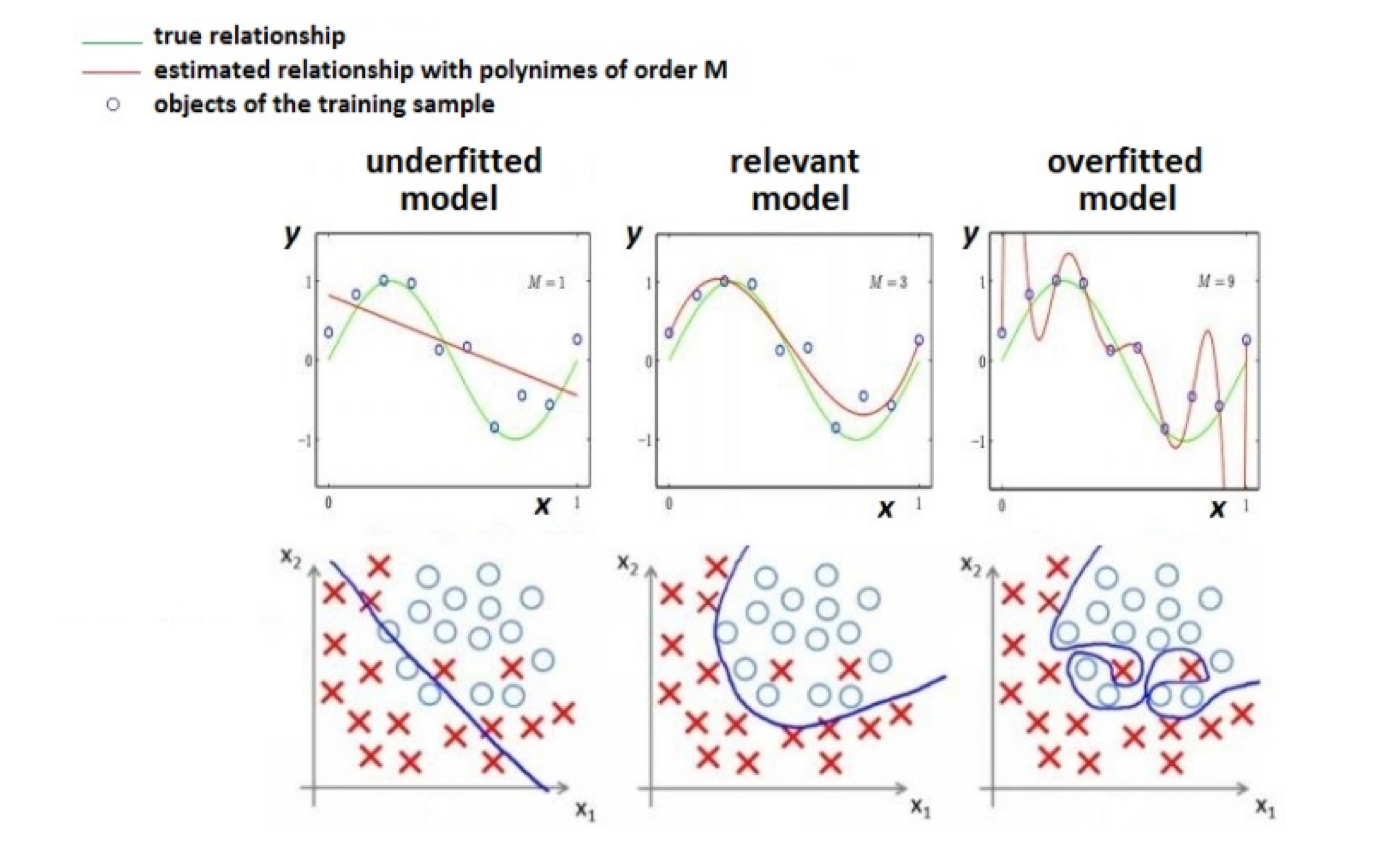
Empirical risk
- Want to minimize expected risk: $$ \mathit{\int}\int\mathit{\mathcal{L}(f_{\theta}(\mathbf{x}),y) \cdot p(\mathbf{x},y)d\mathbf{x}dy\to\min_{\theta}} $$
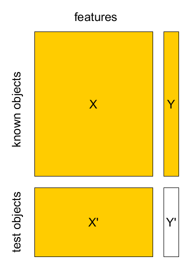
In fact we have only $X$,$Y$ (Known set) and $X'$ (Test set)
Can minimize empirical risk $$ L(\theta|X,Y)=\frac{1}{N}\sum_{n=1}^{N}\mathcal{L}(f_{\theta}(\mathbf{x}_{n}),\,y_{n}) $$
Method of empirical risk minimization: $$ \widehat{\theta}=\arg\min_{\theta}L(\theta|X,Y) $$
- How to get realistic estimate of $L(\widehat{\theta}|X',Y')$?
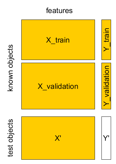
- separate validation set
- cross-validation
- leave-one-out method
Separate validation set
- Known sample $X,Y$: $(\mathbf{x}_{1},y_{1}),...(\mathbf{x}_{M},y_{M})$
- Test sample $X',Y'$: $(\mathbf{x}_{1}',y_{1}'),...(\mathbf{x}_{K}',y_{K}')$
Cross-validation
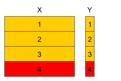
4-fold cross-validation example
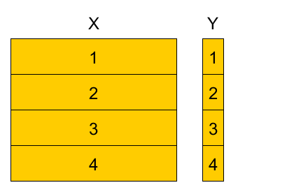
Divide training set into K parts, referred as folds (here $K=4$).
Variants:
- randomly
- randomly with stratification (w.r.t target value or feature value)
- randomly with respect to time domain
- etc
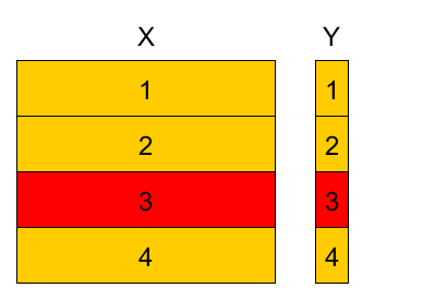
4-fold cross-validation example
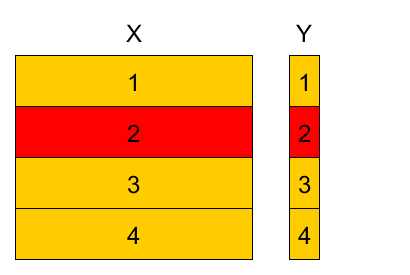
4-fold cross-validation example
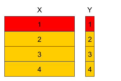
4-fold cross-validation example
4-fold cross-validation example
4-fold cross-validation example
- Denote
- $k(n)$ - fold to which observation $(\mathbf{x}_{n},y_{n})$ belongs $n\in I_{k}$.
- $\widehat{\theta}^{-k}$ - parameter estimation using observations from all folds except fold $k$.
Cross-validation empirical risk estimation
$$\widehat{L}_{total}=\frac{1}{N}\sum_{n=1}^{N}\mathcal{L}(f_{\widehat{\theta}^{-k(n)}}(x_{n}),\,y_{n})$$For $K$-fold CV we have:
- $K$ parameters $\widehat{\theta}^{-1},...\widehat{\theta}^{-K}$
- $K$ models $f_{\widehat{\theta}^{-1}}(\mathbf{x}),...f_{\widehat{\theta}^{-K}}(\mathbf{x}).$
$K$ estimations of empirical risk: $\widehat{L}_{k}=\frac{1}{\left|I_{k}\right|}\sum_{n\in I_{k}}\mathcal{L}(f_{\widehat{\theta}^{-k}}(\mathbf{x}_{n}),\,y_{n}),\,k=1,2,...K.$
- can estimate variance & use statistics!
Comments on cross-validation
- When number of folds $K$ is equal to number of objects $N$, this is called leave-one-out method.
- Cross-validation uses the i.i.d.(independent and identically distributed) property of observations
- Stratification by target $y$ helps for imbalanced/rare classes.
A/B testing
A/B testing
- Observe test set after the models were built.
- A/B testing procedure:
- divide test objects randomly into two groups - A and B.
- apply base model to A
- apply modified model to B
- compare final results\pause
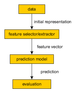
Modelling Pipelines
General Modelling Pipeline
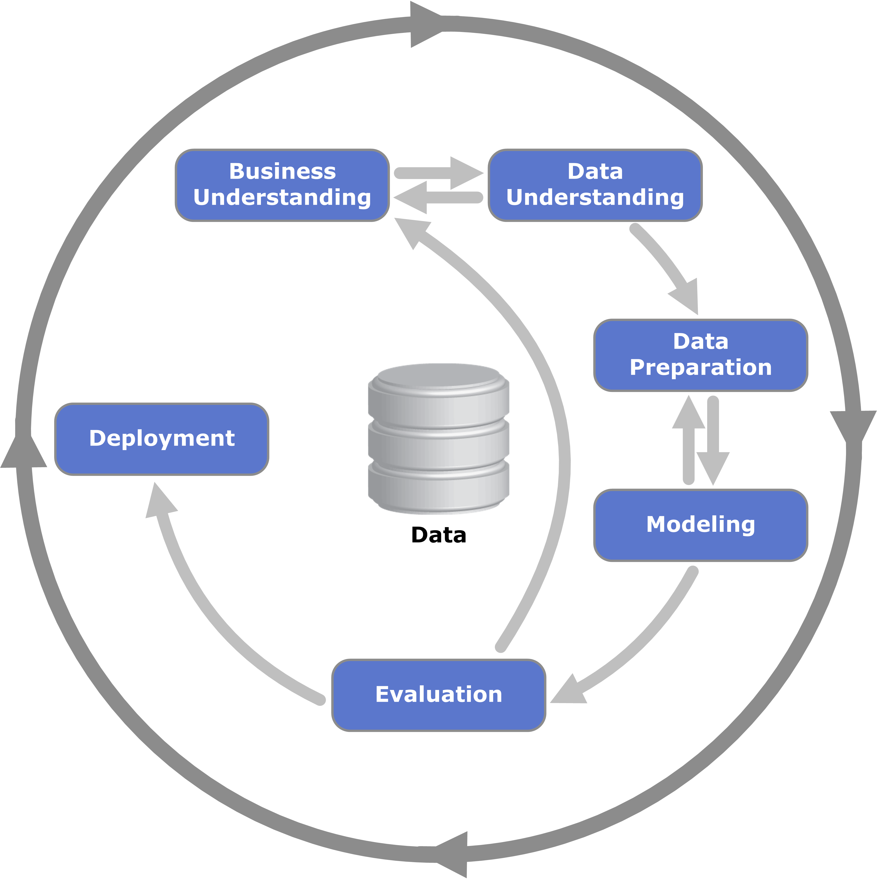
CRISP DM
Metric-based models
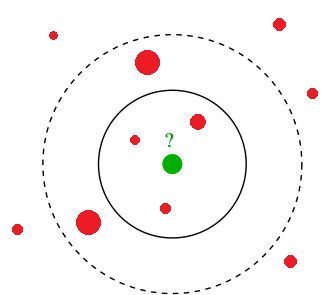
Cluster hypothesis (Compactness hypothesis)
- the more $x$'s features are similar to ones of $x_i$'s, the more likely $\hat{y}=y_i$
Cluster hypothesis examples
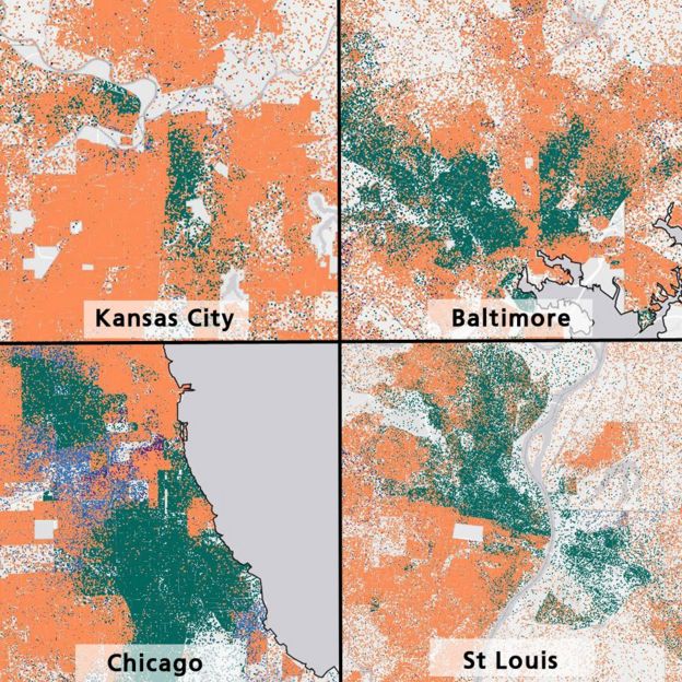
- Objects: Families, households
- Featuers: address, zip code, nearest marketplace... $\rightarrow$ geo-coordinates
(lat, lon) - Target feature: race (classification)
Cluster hypothesis examples
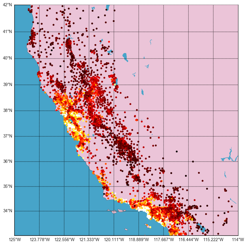
- Objects: Houses
- Features: address... $\rightarrow$ geo-coordinates
(lat, lon) - Target feature: house price (regression)
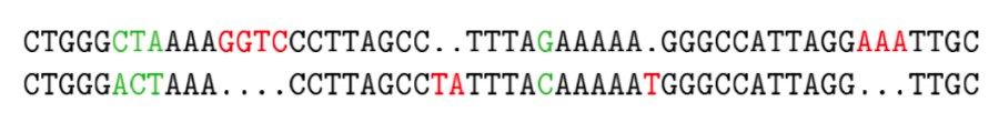
- Objects: DNA strings
- Features: ??
- Target features: Gene function (classification)

- Objects: Documents, texts, articles
- Features: Word counts
- Target: Document category (classification)
Similarity (distance) measures
Similarity measures
- How do we find similar objects?
- Utilize some similiarity measure (could be metric)
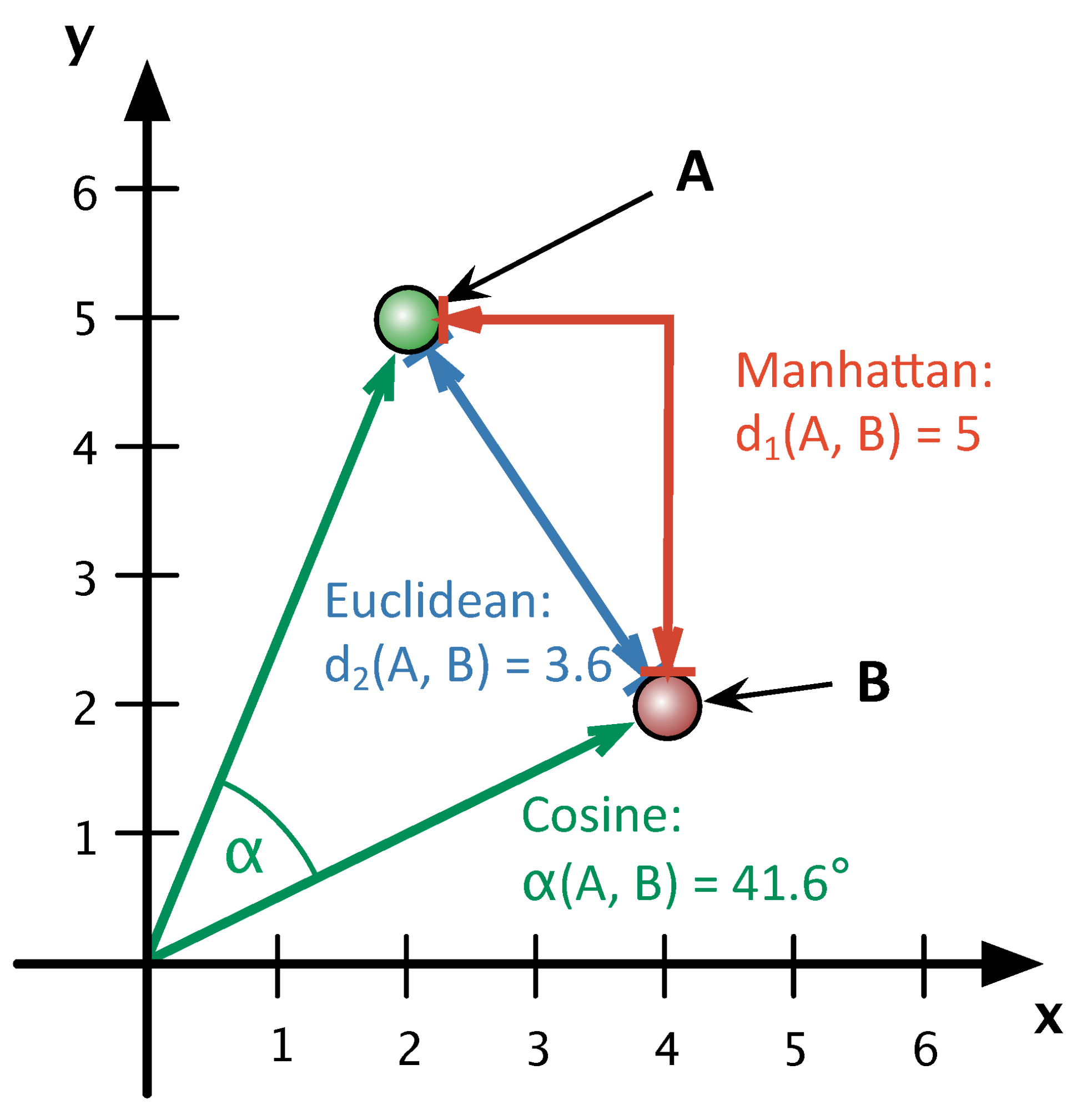
Most popular are
$$ \rho(x_i, x_j) = \sqrt{\sum\limits_{d=1}^{D}(x^d_i - x^d_j)^2} \text{: euclidean distance} $$$$ \rho(x_i, x_j) = \sum\limits_{d=1}^{D}|x^d_i - x^d_j| \text{: manhattan distance} $$$$ \rho(x_i, x_j) = 1 - \frac{\langle x_i,x_j \rangle}{||x_i||_2\cdot||x_j||_2} \text{: cosine distance} $$Illustration
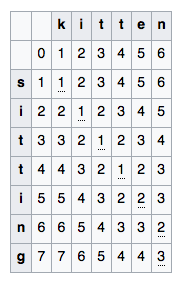
String Similarity
- Edit distance
- Number of insertions, replacements and deletions required to modify string $S_1$ to string $S_2$
- Denote $D( i , j )$ as edit distance between substrings $S_1[:i]$ and $S_2[:j]$.
- Use dynamic programming approach to compute $\rho(S_1, S_2):$
where $m(a,b) = 0$, if $a = b$ and $1$ otherwise
- Jaro–Winkler distance
- ...
Edit distance example
Similarity between sets
- Suppose thet objects are represented with sets
- Client $a$: {french fries, big-mac, coffe, muffin}
- Client $b$: {french fries, cheese sause, cheeseburger, coffe, cherry pie}
- Jaccard distance: $$\rho(a,b) = 1 - \frac{|a \cap b|}{|a \cup b|}$$
Nearest Centroid
Nearest centroids algorithm
Consider training sample $\left(x_{1},y_{1}\right),...\left(x_{N},y_{N}\right)$ with
- $N_{1}$ representatives of 1st class
- $N_{2}$ representatives of 2nd class
- etc.
Training: Calculate centroids for each class $c=1,2,...C:$ $$ \mu_{c}=\frac{1}{N_{1}}\sum_{n=1}^{N}x_{n}\mathbb{I}[y_{n}=c] $$
Classification:
- For object $x$ find the most closest centroid: $$ c=\arg\min_{i}\rho(x,\mu_{i}) $$
- Associate $x$ the class of the most close centroid: $$ \widehat{y}(x)=c $$
Decision boundaries for 4-class nearest centroids}
interact(plot_centroid_class)
Questions
- What are discriminant functions $g_{c}(x)$ for nearest centroid?
- What is the complexity for:
- training?
- prediction?
- What would be the shape of class separating boundary?
- Can we use similar ideas for regression?
- Is it always possible to have centroids?
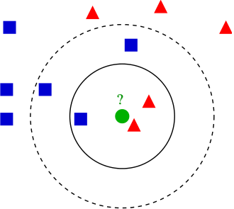
K-nearest neighbours (KNN)
K-nearest neighbours algorithm
Classification:
- Find $k$ closest objects to the predicted object $x$ in the training~set.
- Associate $x$ the most frequent class among its $k$ neighbours.
plt.scatter(X_moons[:,0], X_moons[:,1], c=y_moons, cmap=plt.cm.Spectral)
plt.xlabel('$x_1$')
plt.ylabel('$x_2$')

interact(plot_knn_class, k=IntSlider(min=1, max=10, value=1))
K-nearest neighbours algorithm
Regression:
- Find $k$ closest objects to the predicted object $x$ in the training~set.
- Associate $x$ average output of its $k$ neighbours.
plt.plot(x_true, y_true, c='g', label='$f(x)$')
plt.scatter(x, y, label='actual data')
plt.xlabel('x')
plt.ylabel('y')
plt.legend(loc=2)

plot_linreg()

interact(plot_knn, k=IntSlider(min=1, max=10, value=1))
Comments
- K nearest neighbours algorithm is abbreviated as K-NN.
- $k=1$: nearest neighbour algorithm
- Base assumption of the method:
- similar objects yield similar outputs
- what is simpler - to train K-NN model or to apply it?
Dealing with similar rank
When several classes get the same rank, we can assign to class:
- with higher prior probability
- having closest representative
- having closest mean of representatives (among nearest neighbours)
- which is more compact, having nearest most distant representative
Parameters and modifications
- Parameters:
* None
- Hyperparameters
- the number of nearest neighbours $K$
- distance metric $\rho(x,x')$
- Modifications:
- forecast rejection option (propose a rule, under what conditions to apply rejection in a) classification b) regression)
- variable $K$ (propose a method of K-NN with adaptive variable K in different parts of the feature space)
Properties
Advantages:
- only similarity between objects is needed, not exact feature values.
- so it may be applied to objects with arbitrary complex feature description
- simple to implement
- interpretable (kind of.. case based reasoning)
- does not need training
- may be applied in online scenarios
- cross-validation may be replaced with LOO.
- only similarity between objects is needed, not exact feature values.
- Disadvantages:
- slow classification with complexity $O(NDK)$
- accuracy deteriorates with the increase of feature space dimensionality (curse of dimentionality)
Special properties
Normalization of features
- Feature scaling affects predictions of K-NN?
Normalization of features
- Feature scaling affects predictions of K-NN?
- sure it does! Need to normalize
- Equal scaling - equal impact of features
- Non-equal scaling - non-equal impact of features
- Typical normalizations:
- z-scoring (autoscaling): $$x_{j}'=\frac{x_{j}-\mu_{j}}{\sigma_{j}}$$
- range scaling: $$x_{j}'=\frac{x_{j}-L_{j}}{U_{j}-L_{j}}$$
where $\mu_{j},\,\sigma_{j},\,L_{j},\,U_{j}$ are mean value, standard deviation, minimum and maximum value of the $j$-th feature.
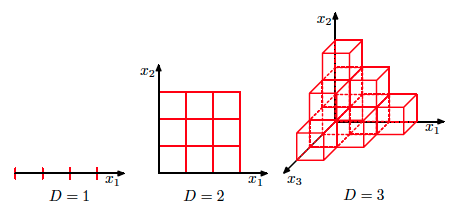
The curse of dimensionality
- Phenomenon that occures in various fields and have varoius consequences (mainly negative)
- The curse of dimensionality: with growing $D$ data distribution becomes sparse and insufficient.
The curse of dimensionality
- At what rate should training size grow with increase of $D$ to compensate curse of dimensionality?
The curse of dimensionality
$D=2$ |
$D=2 \dots 100$ |
|---|
Curse of dimensionality
- Case of K-nearest neighbours:
- assumption: objects are distributed uniformly in unit feature space
- ball of radius $R$ has volume $V(R)=CR^{D}$, where $C=\frac{\pi^{D/2}}{\Gamma(D/2+1)}$.
- ratio of volumes of unit cube and included ball: $$ \frac{V(0.5)}{1}=\frac{0.5^{D}\pi^{D/2}}{(D/2)!}\stackrel{D\to\infty}{\longrightarrow}0 $$
- most of volume concentrates on the corners of the cube
- nearest neighbours stop being close by distance
- Good news: in real tasks the true dimensionality of the data is often less than $D$ and objects belong to the manifold with smaller dimensionality.
Weighted account
Equal voting
Consider for object $x$:
- $x_{i_{1}}$most close neigbour, $x_{i_{2}}$ - second most close neighbour, etc. $$ \rho(x,x_{i_{1}})\le\rho(x,x_{i_{2}})\le...\le\rho(x,x_{i_{N}}) $$
Classification: $$\begin{align*} g_{c}(x) & =\sum_{k=1}^{K}\mathbb{I}[y_{i_{k}}=c],\quad c=1,2,...C.\\ \widehat{y}(x) & =\arg\max_{c}g_{c}(x) \end{align*} $$
Regression: $$ \widehat{y}(x)=\frac{1}{K}\sum_{k=1}^{K}y_{i_{k}} $$
Weighted voting
Weighted classification: $$\begin{align*} g_{c}(x) & =\sum_{k=1}^{K}w(k,\,\rho(x,x_{i_{k}}))\mathbb{I}[y_{i_{k}}=c],\quad c=1,2,...C.\\ \widehat{y}(x) & =\arg\max_{c}g_{c}(x) \end{align*} $$
Weighted regression: $$ \widehat{y}(x)=\frac{\sum_{k=1}^{K}w(k,\,\rho(x,x_{i_{k}}))y_{i_{k}}}{\sum_{k=1}^{K}w(k,\,\rho(x,x_{i_{k}}))} $$
Commonly chosen weights
Index dependent weights: $$ w_{k}=\alpha^{k},\quad\alpha\in(0,1) $$ $$ w_{k}=\frac{K+1-k}{K} $$
Distance dependent weights:
$$ w_{k}=\begin{cases} \frac{\rho(z_{K},x)-\rho(z_{k},x)}{\rho(z_{K},x)-\rho(z_{1},x)}, & \rho(z_{K},x)\ne\rho(z_{1},x)\\ 1 & \rho(z_{K},x)=\rho(z_{1},x) \end{cases} $$$$ w_{k}=\frac{1}{\rho(z_{k},x)} $$Kernels
- $K(\rho, h)$ - some decreasing function
- $h \geq 0$ - parameter (window width)
- gaussian kernel $$K(\rho, h) \propto \exp(- \frac{\rho(x, x')^2}{2h^2})$$
- tophat kernel $$K(\rho, h) \propto 1\ if\ x < h$$
- epanechnikov kernel $$K(\rho, h) \propto 1 - \frac{\rho(x, x')^2}{h^2}$$
- exponential kernel $$K(\rho, h) \propto \exp(-\rho(x, x')/h)$$
- linear kernel $$K(\rho, h) \propto 1 - \rho(x, x')/h\ if\ d < h$$
Kernels

interact(plot_knn_class_kernel, k=IntSlider(min=1, max=10, value=1),
               h=FloatSlider(min=0.05, max=5, value=1, step=0.05))
Summary
Important hyperparameters of K-NN:
- $K$: controls model complexity
- $\rho(x,x')$
Output depends on feature scaling.
- scaling to equal / non-equal scatter possible.
- Prone to curse of dimensionality.
- Fast training but long prediction.
- some efficiency improvements are possible though
- Weighted account for objects possible.
Use Case
- Despite being very primitive KNN demonstrated good performance in Facebook's Kaggle competiton
- Used to make features
- Competiton page
- Winner interview