Data Analysis
Andrey Shestakov (avshestakov@hse.ru)
Decision trees1
1. Some materials are taken from machine learning course of Victor Kitov
Let's recall previous lecture
- Metric methods: Nearest Centroid, K Nearest Neighbours
- Work both for classification and regression
- Lazy learning - simply remember training dataset
- No parameters - only hyper-parameters
- Cluster hypothesis - the core of metric methods
- Similarity measures and distances: euclidean, cosine, edit-distance, Jaccard similarity, etc...
- Feature scaling is important!
- Various modifications:
- weighted domain
- work on "tied" cases
- adaptive K
- ...
- Get ready to face with
- Curse of dimentionality
- Slow prediction speed
Decision trees
Intuition
Intuition 1
- A perfumery company developed a new unisex smell
- To find their key segments it they run open world testing
- Each respondent leaves
- responce if she likes it or not (
+1|-1) - some info about her
- Gender
- Age
- Education
- Current career
- Have domestic animals
- etc..
- responce if she likes it or not (
Intuition 1
In the end the description of the segments could look like this
[Gender = F][Age > 21][Age <= 25][Education = Higher][Have domestic animals = No]- like in 82% of cases[Gender = M][Age > 25][Age <= 30][Current Career = Manager]- don't like in 75% of cases- ...
Intuition 2
- You are going to take a loan
god, please, noto buy something expensive, and provide your application form - Bank employee is checking it accoring to some rules like:
- Current bank account > 200k rubles. - go to step 2, otherwise 3
- Duration < 30 months - go to step 4, otherwise REJECT
- Current employment > 1 year - ACCEPT, otherwise REJECT
- ...
Intuition 2

Intuition 3

Intuition 4
Intuition 4


Definition of decision tree
Prediction is performed by tree $T$ (directed, connected, acyclic graph)
Node types
- A root node, $root(T)$
- Internal nodes $int(T)$, each having $\ge2$ child nodes
- Terminal nodes (leafs), $terminal(T)$, which do not have child nodes but have associated prediction values
Definition of decision tree
- for each non-terminal node $t$ a check-function $Q_{t}(x)$ is associated
- for each edge $r_{t}(1),...r_{t}(K_{t})$ a set of values of check-function
$Q_{t}(x)$ is associated: $S_{t}(1),...S_{t}(K_{t})$ such that:
- $\bigcup_{k}S_{t}(k)=range[Q_{t}]$
- $S_{t}(i)\cap S_{t}(j)=\emptyset$ $\forall i\ne j$
Prediction process
- Prediction is easy if we have already constructed a tree
Prediction process for tree $T$:
- $t=root(T)$
while $t$ is not a terminal node:
- calculate $Q_{t}(x)$
- determine $j$ such that $Q_{t}(x)\in S_{t}(j)$
- follow edge $r_{t}(j)$ to $j$-th child node: $t=\tilde{t}_{j}$
- return prediction, associated with leaf $t$.
Specification of decision tree
- To define a decision tree one needs to specify:
- the check-function: $Q_{t}(x)$
- the splitting criterion: $K_{t}$ and $S_{t}(1),...S_{t}(K_{t})$
- the termination criteria (when node is defined as a terminal node)
- the predicted value for each leaf node.
Genralized decision tree algorithm
{python}
1. function decision_tree(X, y):

2.    if termination_criterion(X, y) == True:

3.        S = create_leaf_with_prediction(y)

4.    else:

5.        S = create_node()
6.        (X_1, y_1) .. (X_L, y_L) = best_split(X, y)

7.        for i in 1..L:
8.            C = decision_tree(X_i, y_i)
9.            connect_nodes(S, C)
10.   return S
Splitting rules
Possible definitions of splitting rules
- $Q_{t}(x)=x^{i(t)}$, where $S_{t}(j)=v_{j}$, where $v_{1},...v_{K}$ are unique values of feature $x^{i(t)}$.
- $S_{t}(1)=\{x^{i(t)}\le h_{t}\},\,S_{t}(2)=\{x^{i(t)}>h_{t}\}$
- $S_{t}(j)=\{h_{j}<x^{i(t)}\le h_{j+1}\}$ for set of partitioning thresholds $h_{1},h_{2},...h_{K_{t}+1}$.
- $S_{t}(1)=\{x:\,\langle x,v\rangle\le0\},\quad S_{t}(2)=\{x:\,\langle x,v\rangle>0\}$
- $S_{t}(1)=\{x:\,\left\lVert x\right\rVert \le h\},\quad S_{t}(2)=\{x:\,\left\lVert x\right\rVert >h\}$
- etc.
Most famous decision tree algorithms
- C4.5
- ID 3
- CART (classification and regression trees)
- implemented in scikit-learn (kind of)
CART version of splitting rule
- single feature value is considered: $$ Q_{t}(x)=x^{i(t)} $$
- binary splits: $$ K_{t}=2 $$
- split based on threshold $h_{t}$: $$ S_{1}=\{x^{i(t)}\le h_{t}\},\,S_{2}=\{x^{i(t)}>h_{t}\} $$
$h(t)\in\{x_{1}^{i(t)},x_{2}^{i(t)},...x_{N}^{i(t)}\}$
- applicable only for real, ordinal and binary features
- what about categorical features?
Splitting rule selection
Classification impurity functions
- For classification: let $p_{1},...p_{C}$ be class probabilities for objects in node $t$.
Then impurity function $\phi(t)=\phi(p_{1},p_{2},...p_{C})$ should satisfy:
- $\phi$ is defined for $p_{j}\ge0$ and $\sum_{j}p_{j}=1$.
- $\phi$ attains maximum for $p_{j}=1/C,\,k=1,2,...C$ .
- $\phi$ attains minimum when $\exists j:\,p_{j}=1,\,p_{i}=0$ $\forall i\ne j$.
- $\phi$ is symmetric function of $p_{1},p_{2},...p_{C}$.
Typical classification impurity functions}
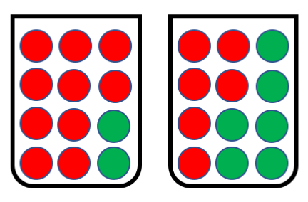
Gini criterion
- interpretation: probability to make mistake when predicting class randomly with class probabilities $[p(\omega_{1}|t),...p(\omega_{C}|t)]$: $$ I(t)=\sum_{i}p(\omega_{i}|t)(1-p(\omega_{i}|t))=1-\sum_{i}[p(\omega_{i}|t)]^{2} $$
Entropy
- interpretation: measure of uncertainty of random variable $$ I(t)=-\sum_{i}p(\omega_{i}|t)\ln p(\omega_{i}|t) $$
Classification error
- interpretation: frequency of errors when classifying with the most common class $$ I(t)=1-\max_{i}p(\omega_{i}|t) $$
plot_impurities()

Splitting criterion selection
Define $\Delta I(t)$ - is the quality of the split of node $t$ into child nodes $t_{1},...t_{C}$. $$ \Delta I(t)=I(t)-\sum_{i=1}^{C}I(t_{i})\frac{N(t_{i})}{N(t)} $$ $$ \Delta I(t)=I(t)-\left(I(t_{L})\frac{N(t_{L})}{N(t)} + I(t_{R})\frac{N(t_{R})}{N(t)}\right) $$
- If $I(t)$ is entropy, then $\Delta I(t)$ is called information gain.
- CART optimization (regression, classification): select feature $i_{t}$ and threshold $h_{t}$, which maximize $\Delta I(t)$: $$ i_{t},\,h_{t}=\arg\max_{k,h}\Delta I(t) $$
- CART decision making: from node $t$ follow:
Splitting criterion selection
Remarks
- Local and Greedy optimization
- Overall results changes slighly with different impurity measures
wine_demo()

Typical regression impurity functions
- Impurity function measures uncertainty in $y$ for objects falling inside node $t$.
- Regression:
- let objects falling inside node $t$ be $I=\{i_{1},...i_{K}\}$. We may define
\begin{align*}
\phi(t) & =\frac{1}{K}\sum_{i\in I}\left(y_{i}-\mu\right)^{2}\quad \text{(MSE)}\\
\phi(t) & =\frac{1}{K}\sum_{i\in I}|y_{i}-\mu|\quad \text{(MAE)}
\end{align*}
where $\mu$ is
meanormedianof $y_i$s.
- let objects falling inside node $t$ be $I=\{i_{1},...i_{K}\}$. We may define
\begin{align*}
\phi(t) & =\frac{1}{K}\sum_{i\in I}\left(y_{i}-\mu\right)^{2}\quad \text{(MSE)}\\
\phi(t) & =\frac{1}{K}\sum_{i\in I}|y_{i}-\mu|\quad \text{(MAE)}
\end{align*}
where $\mu$ is
- Regression:
Prediction assignment to leaves
- Regression:
- mean (optimal for MSE loss)
- median (optimal for MAE loss)
- Classification
- most common class (optimal for constant misclassification cost)
Classification example
fig = interact(demo_dec_tree, depth=IntSlider(min=1, max=5, value=1))
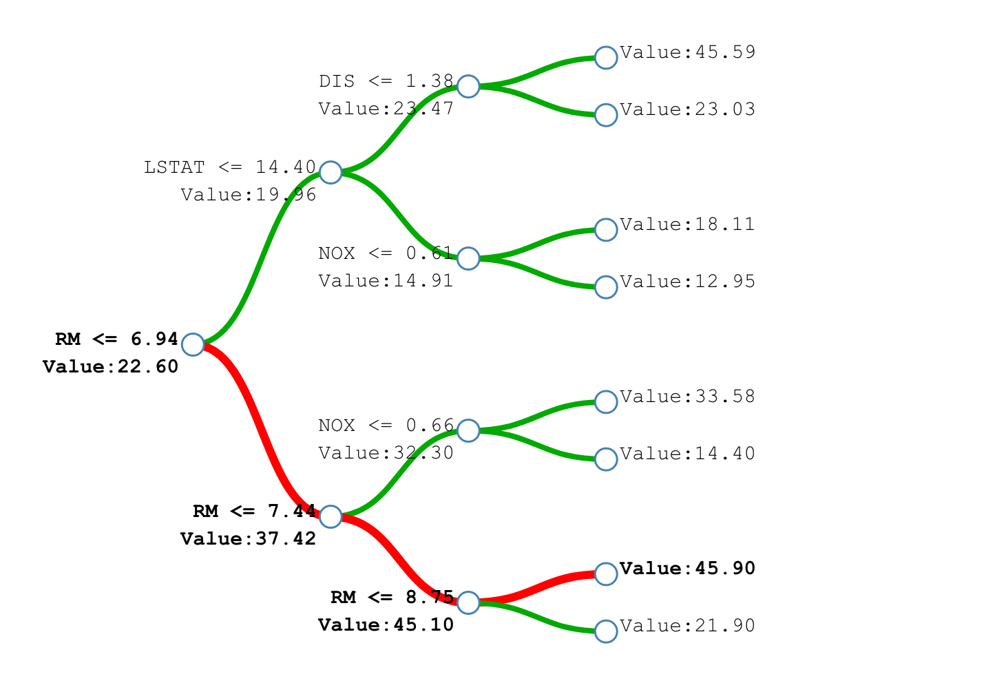
Regression example
fig = interact(plot_dec_reg, depth=IntSlider(min=1, max=5, value=1), criterion=['mse', 'mae'])
Termination criterion
Termination criterion
- Tradeoff:
- very large complex trees -> overfitting
- very short simple trees -> underfitting
- Approaches to stopping:
- rule-based
- based on pruning (not considered here)
Rule-base termination criteria
- Rule-based: a criterion is compared with a threshold.
- Variants of criterion:
- depth of tree
- number of objects in a node
- minimal number of objects in one of the child nodes
- impurity of classes
- change of impurity of classes after the split
- etc
Analysis of rule-based termination
Advantages:
- simplicity
- interpretability
Disadvantages:
- specification of threshold is needed
Other features
Tree feature importances
- Consider feature $f$
- Let $T(f)$ be the set of all nodes, relying on feature $f$ when making split.
- efficiency of split at node $t$: $\Delta I(t)=I(t)-\sum_{c\in childen(t)}\frac{n_{c}}{n_{t}}I(c)$
- feature importance of $f$: $\sum_{t\in T(f)}n_{t}\Delta I(t)$
- Alternative: difference in decision tree prediction quality for
- original validation set
- validation set with $j$-th feature randomly shuffled
Handling missing values
- Remove features or objects with missing values
- Missing value = distinct feature value
- Calculation of impurity w/o missing cases
- Surrogate split!
- Find best split with feature $i^*$, threshold $h^*$ and children $\{t^*_L, t^*_R\}$
- Find other good splits for features $i_t \neq i^*$, s.t. $\{t_L, t_R\} \approx \{t^*_L, t^*_R\}$
- While performing prediction of object $x$:
- If $x^{i^*}$ is
Null, try $x^{i_t}$
- If $x^{i^*}$ is
Analysis of decision trees
Advantages:
- simplicity of algorithm
- interpretability of model (for short trees)
- implicit feature selection
- good for features of different nature:
- naturally handles both discrete and real features
- prediction is invariant to monotone transformations of features
Analysis of decision trees
- Disadvantages:
- not very high accuracy:
- high overfitting of tree structure up to top
- non-parallel to axes class separating boundary may lead to many nodes in the tree for $Q_{t}(x)=x^{i(t)}$
- one step ahead lookup strategy for split selection may be insufficient (XOR example)
- not online - slight modification of the training set will require full tree reconstruction.
- not very high accuracy:
Special Desicion Tree Algorithms
ID 3
- Categorical features only
- Number of children = number of categories
- Maximum depth
С 4.5
- Handling continious features
- And categorical as in ID3
- Find missing value - proceed down to all paths and average
- Some prunning procedure