Data Analysis
Andrey Shetakov (avshestakov@hse.ru)
Linear regression. Gradient-based optimization1
1. Some materials are taken from machine learning course of Victor Kitov
Let's recall previous lecture
- Decision trees
- Utilize the notion of impurity
- Work both for classification and regression
- Implicit feature selection
- good for features of different nature
- Parallel to axes class separating boundary
- Local greedy optimizaion
- Sensitive to even tiny data pertubations
Linear regression
Example: flat prices
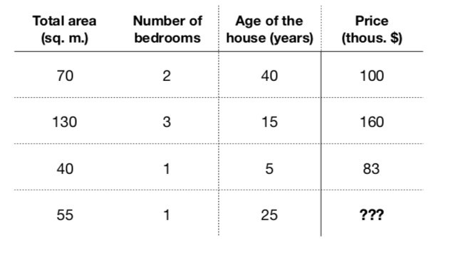
- Obviously, those characteristics somehow relate with price ($f: X \rightarrow Y$)
- Formalize a model to predict flat price: $$a(x) = a(total\_area, nmbr\_of\_bedrooms, house\_age) = \hat{y}$$
- Let it be a linear model: $$a(x) = \beta_0 + \beta_1\cdot total\_area + \beta_2 \cdot nmbr\_of\_bedrooms + \beta_3 \cdot house\_age$$
- Learning - find coefficients $\beta_0,\dots, \beta_3$, that minimizer error on training set
Cars price vs mileage
df_auto.plot(x='mileage', y='price', kind='scatter')

Linear regression
- Our goal - determine linear dependence between features $X$ and target vector $y$
- Define $x_n^d$ as $d$-th feature of $n$-th object, $y_{n} \in \mathbb{R}$ - target value for $n$-th object $$f(x_{n}, \beta) = \hat{y}_{n} = \beta_0 + \beta_1x_{n}^1 + \dots$$
- $x_{n}^0 = 1$ $\forall n$ - intercept
- Need to estimate $\beta_i$.
Ordinary Least Squares: $$ L(\beta_0,\beta_1,\dots) = \frac{1}{2N}\sum^{N}_{n=1}(\hat{y}_{n} - y_{n})^2 = \frac{1}{2N}\sum^{N}_{n=1}\left(\sum_{d=0}^{D}\beta_{d}x_{n}^{d}-y_{n}\right)^{2} \rightarrow \min\limits_{\beta} $$
Solution
Let's say $f(x, \beta) = \beta_0 + \beta_1x_1$
Calculate partial derivatives wrt $\beta_0$, $\beta_1$ and set them to $0$:
$$ \frac{\partial L}{\partial \beta_0} = \frac{1}{N}\sum^{N}_{n=1}(\beta_0 + \beta_1x_{n}^1 - y_{n}) = 0$$$$ \frac{\partial L}{\partial \beta_1} = \frac{1}{N}\sum^{N}_{n=1}(\beta_0 + \beta_1x_{n}^1 - y_{n})x^1_{n} = 0$$Linear regression (in matrix form)
- Define $X\in\mathbb{R}^{NxD},\{X\}_{ij}$ defines the $j$-th feature of $i$-th object, $y\in\mathbb{R}^{n}$ - vector with target values $$f(x, \beta) = \hat{y} = X\beta \quad \Leftrightarrow \quad \left( \begin{array}{c} \hat{y}_1 \\ \hat{y}_2 \\ \vdots \\ \hat{y}_n \end{array} \right) = \left( \begin{array}{ccccc} 1 & x_1^1 & x_1^2 & \cdots & x_1^d\\ 1 & x_2^1 & x_2^2 & \cdots & x_2^d\\ \cdots & \cdots & \cdots & \cdots & \cdots\\ 1 & x_n^1 & x_n^2 & \cdots & x_n^d\end{array} \right) \cdot \left( \begin{array}{c} \beta_0 \\ \beta_1 \\ \vdots\\ \beta_d \end{array} \right) $$
- Need to estimate $\beta_i$.
Ordinary Lears Squares: $$ L(\beta) = \frac{1}{2N}(\hat{y} - y)^{\top}(\hat{y} - y) = \frac{1}{2N}(X\beta - y)^{\top}(X\beta - y) \rightarrow \min\limits_{\beta} $$
Solution (in matrix form)
Expand a bit $$ \begin{align*} L(\beta) & = \frac{1}{2N}(X\beta - y)^{\top}(X\beta - y) \\ & = \frac{1}{2N}\left( \beta^\top X^\top X \beta - 2 (X\beta)^\top y + y^\top y \right) \end{align*} $$
Calculate vector of partial derivatives - gradient
Comments
- This is the global minimum, because the optimized criteria is convex.
- Geometric interpretation:
- find linear combination of feature measurements that best reproduce $y$
- solution - combinaton of features, giving projection of $y$ on linear span of feature measurements.
- Why using Normal Equation could be bad?
- Calculating inverse costs a lot
- Not all matrices have it (singular matrices)
Linearly dependent features (multicollinearity)
- Solution $\widehat{\beta}=(X^{T}X)^{-1}X^{T}y$ exists when $X^{T}X$ is non-singular
- Problem occurs when one of the features is a linear combination of the other (linear dependency)
- interpretation: non-identifiability of $\widehat{\beta}$ for linearly dependent features:
- linear dependence: $\exists\alpha:\,x^{T}\alpha=0\,\forall x$
- suppose $\beta$ solves linear regression $y=x^{T}\beta$
- then $x^{T}\beta\equiv x^{T}\beta+kx^{T}\alpha\equiv x^{T}(\beta+k\alpha)$, so $\beta+k\alpha$ is also a solution!
- interpretation: non-identifiability of $\widehat{\beta}$ for linearly dependent features:
- Multicollinearity can be exact and not exact, which is also bad
Examples of linear dependency
- $x$ miles $\approx 1.6\cdot x$ kms
- total flat area $\approx$ area of living rooms $+$ area of kitchen
- dummy variable trap!
Linearly dependent features
- Problem may be solved by:
- feature selection
- dimensionality reduction
- imposing additional requirements on the solution (regularization)
Analysis of linear regression
Advantages:
- single optimum, which is global (for non-singular matrix)
- analytical solution
- interpretable solution and algorithm
Drawbacks:
- too simple model assumptions (may not be satisfied)
- $X^{T}X$ should be non-degenerate (and well-conditioned)
Intuition
$$ L(\beta_0, \beta_1) = \frac{1}{2N}\sum_{n=1}^N(\beta_0 + \beta_1x^1_{n} - y_{n})^2$$- Suppose we have some initial approximation of $(\hat{\beta_0}, \hat{\beta_1})$
- How should we change it in order to improve?
sq_loss_demo()

Tiny Refresher
Derivative of $f(x)$ in $x_0$: $$ f'(x_0) = \lim\limits_{h \rightarrow 0}\frac{f(x_0+h) - f(x_0)}{h}$$
Derivative shows the slope of tangent line in $x_0$
- If $x_0$ is extreme point of $f(x)$ and $f'(x_0)$ exists $\Rightarrow$ $f'(x_0) = 0$
interact(deriv_demo, h=FloatSlider(min=0.0001, max=2, step=0.005), x0=FloatSlider(min=1, max=15, step=.2))
Tiny Refresher
- In multidimential world we switch to gradients and directional derivatives: $$ f'_v(x_0) = \lim\limits_{h \rightarrow 0}\frac{f(x_0+hv) - f(x_0)}{h} = \frac{d}{dh}f(x_{0,1} + hv_1, \dots, x_{0,d} + hv_d) \rvert_{h=0}, \quad ||v|| = 1 \quad \text{directional derivatives}$$
Tiny Refresher
- Unsing multivariate chain rule:
Tiny Refresher
$$ \langle \nabla f, v \rangle = || \nabla f || \cdot \cos{\phi}$$- Directional derivative is maximal what direction is collinear to gradient
- gradient — direction of steepest ascent of $f(x)$
- antigradient — direction of steepest descent of $f(x)$
Given $L(\beta_0, \beta_1)$ calculate gradient (patial derivatives) $$ \frac{\partial L}{\partial \beta_0} = \frac{1}{N}\sum^{N}_{i=1}(\beta_0 + \beta_1x_{n}^1 - y^{n})$$ $$ \frac{\partial L}{\partial \beta_1} = \frac{1}{N}\sum^{N}_{i=1}(\beta_0 + \beta_1x_{n}^1 - y^{n})x^1_{n}$$
Or in matrix form: $$ \nabla_{\beta}L(\beta) = \frac{1}{N} X^\top(X\beta - y)$$
Run gradient update, which is simultaneous(!!!) update of $\beta$ in antigradient direction:
$$ \beta := \beta - \alpha\nabla_{\beta}L(\beta)$$- $\alpha$ - descent "speed"
Pseudocode
{python}
1.function gd(X, alpha, epsilon):

2.  initialise beta

3.  do:

4.      Beta = new_beta

5.      new_Beta = Beta - alpha*grad(X, beta)

6.  until dist(new_beta, beta) < epsilon

7. return betagrad_demo(iters=105, alpha=0.08)

Comments
- How do we set $\alpha$
- Feature scales matters

- Local minima*


Stochastic gradient descent
{python}
1.function sgd(X, alpha, epsilon):

2.  initialise beta

3.  do:

4.        X = shuffle(X)

5.        for x in X:

6.            Beta = new_beta

7.            new_Beta = Beta - alpha*grad(x, beta)

8.  until dist(new_beta, beta) < epsilon

9. return betastoch_grad_demo(iters=105, alpha=0.08)

Momentum
Idea: to move not only to current antigradient direction but consider previous one
$$ v_0 = 0$$$$ v_t = \gamma v_{t - 1} + \alpha\nabla_{\beta}{L(\beta)}$$$$ \beta = \beta - v_t$$where
- $\gamma$ — momentum term (usually 0.9)
Adagrad
Idea: update parameters $\beta_i$ for each feature differenly.
Denote $\frac{\partial L}{\partial \beta_i}$ on iteration $t$ as $g_{t,i}$
Vanilla gd update
$$ \beta_{t+1, i} = \beta_{t, i} - \alpha \cdot g_{t,i}$$In Adagrad $\alpha$ is normalized wrt "size" of previous derivatives:
$$ \beta_{t+1, i} = \beta_{t, i} - \dfrac{\alpha}{\sqrt{G_{t,ii} + \varepsilon}} \cdot g_{t,i}$$where $G_t$ is diagonal matrix with sum of squares of derivatives of $\beta_{i}$ before iteration $t$. $\varepsilon$ — is smoothing hyperparameter.
FYI
- Zero-order methods
- like...
- 2nd order methods
- Newton method
Nonlinear dependencies
Generalization by nonlinear transformations
Nonlinearity by $x$ in linear regression may be achieved by applying non-linear transformations to the features:
$$ x\to[\phi_{0}(x),\,\phi_{1}(x),\,\phi_{2}(x),\,...\,\phi_{M}(x)] $$$$ f(x)=\mathbf{\phi}(x)^{T}\beta=\sum_{m=0}^{M}\beta_{m}\phi_{m}(x) $$The model remains to be linear in $\beta$, so all advantages of linear regression remain.
Typical transformations
- $x^{i}\in[a,b]$ : binarization of feature
- $x^{i}x^{j}$ : interaction of features
- $\exp\left\{ -\gamma\left\lVert x-\tilde{x}\right\rVert ^{2}\right\} $ : closeness to reference point $\tilde{x}$
- $\ln x_{k}$ : the alignment of the distribution with heavy tails
demo_weights()
