Data Analysis
Andrey Shestakov (avshestakov@hse.ru)
Regularization in linear models.
Linear classification. Logistic Regression1
1. Some materials are taken from machine learning course of Victor Kitov

Let's recall previous lecture
- Linear regression
- linear dependence between target features and predictors
- Optimize Ordinary Least Squares
- Solution can be found
- analytically
- with gradient descent
df_auto.plot(x='mileage', y='price', kind='scatter')

from sklearn.linear_model import LinearRegression
X = df_auto.loc[:,['mileage']].values
y = df_auto.loc[:, 'price'].values

model = LinearRegression()
model.fit(X, y)
print('price = {:.2f} {:.2f}*mileage'.format(model.intercept_, model.coef_[0]))
df_auto.loc[:, 'kilometerage'] = df_auto.loc[:,'mileage'] * 1.60934
X = df_auto.loc[:,['mileage', 'kilometerage']].values
y = df_auto.loc[:, 'price'].values

model = LinearRegression()
model.fit(X, y)
print('price = {:.2f} {:.2f}*mileage {:.2f}*kilometerage'.format(model.intercept_, *model.coef_))
Regularization & restrictions
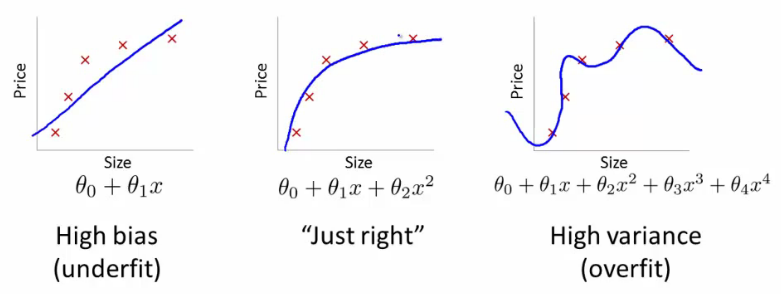
Intuition
Regularization
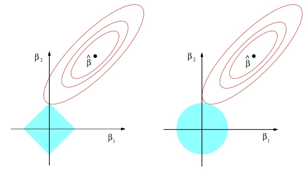
- Insert regularizer $R(\beta)$ for $\beta$ to be small: $$ \sum_{n=1}^{N}\left(x_{n}^{T}\beta-y_{n}\right)^{2}+\lambda R(\beta)\to\min_{\beta} $$
- $\lambda>0$ - hyperparameter.
$R(\beta)$ penalizes complexity of models. $$ \begin{array}{ll} R(\beta)=||\beta||_{1} & \mbox{Lasso regression}\\ R(\beta)=||\beta||_{2}^{2} & \text{Ridge regression} \end{array} $$
Not only accuracy matters for the solution but also model simplicity!
- $\lambda$ controls complexity of the model:$\uparrow\lambda\Leftrightarrow\text{complexity}$$\downarrow$.
Comments
Dependency of $\beta$ from $\lambda$ for ridge (A) and LASSO (B):
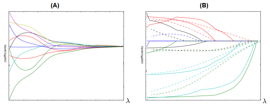
LASSO can be used for automatic feature selection.
- $\lambda$ is usually found using cross-validation on exponential grid, e.g. $[10^{-6},10^{-5},...10^{5},10^{6}]$.
- It's always recommended to use regularization because
- it gives smooth control over model complexity.
- reduces ambiguity for multiple solutions case.
from sklearn.linear_model import Lasso
model = Lasso(alpha=1.)

model.fit(X, y)
print('price = {:.2f} {:.2f}*mileage {:.2f}*kilometerage'.format(model.intercept_, *model.coef_))
ElasticNet
- ElasticNet:
$\alpha\in(0,1)$ - hyperparameter, controlling impact of each part.
- If two features $x^{i}$and $x^{j}$ are equal:
- LASSO may take only one of them
- Ridge will take both with equal weight
- but it doesn't remove useless features
- ElasticNet both removes useless features but gives equal weight for usefull equal features
- good, because feature equality may be due to chance on this particular training set
Different account for different features
- Traditional approach regularizes all features uniformly: $$ \sum_{n=1}^{N}\left(x_{n}^{T}\beta-y_{n}\right)^{2}+\lambda R(\beta)\to\min_{w} $$
- Suppose we have $K$ groups of features with indices: $$ I_{1},I_{2},...I_{K} $$
- We may control the impact of each group on the model by: $$ \sum_{n=1}^{N}\left(x_{n}^{T}\beta-y_{n}\right)^{2}+\lambda_{1}R(\{\beta_{i}|i\in I_{1}\})+...+\lambda_{K}R(\{\beta_{i}|i\in I_{K}\})\to\min_{w} $$
- $\lambda_{1},\lambda_{2},...\lambda_{K}$ can be set using cross-validation
- In practice use common regularizer but with different feature scaling.
Different loss-functions
Idea
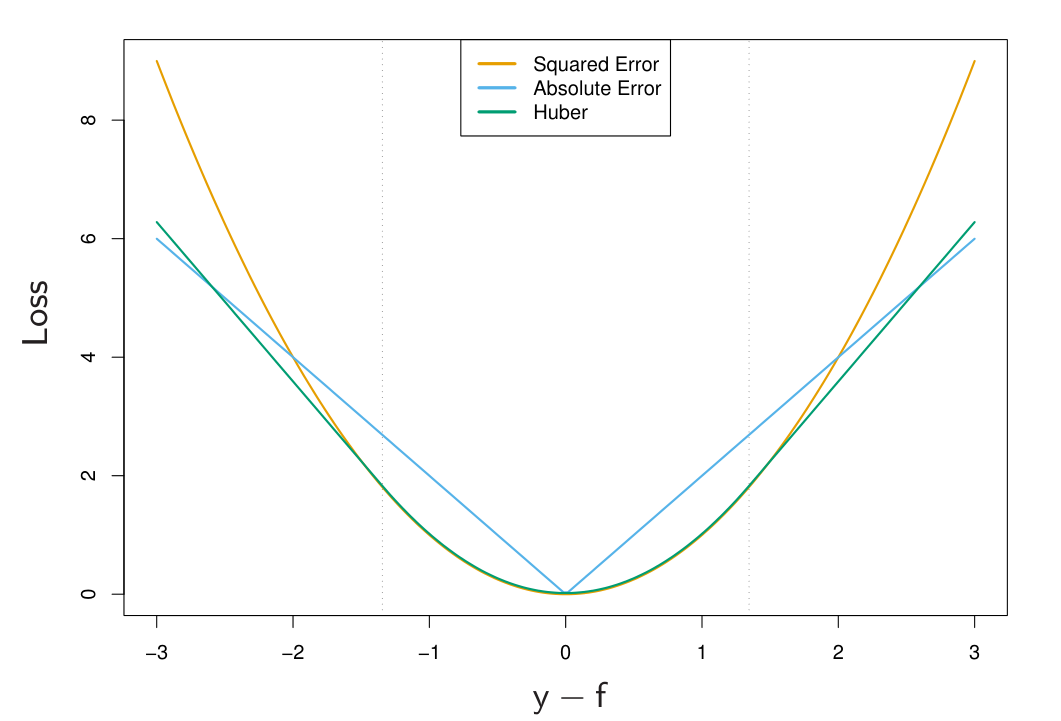
- Generalize squared to arbitrary loss: $$ \sum_{n=1}^{N}\left(x^{T}\beta-y_{n}\right)^{2}\to\min_{\beta}\qquad\Longrightarrow\qquad\sum_{n=1}^{N}\mathcal{L}(x_{n}^{T}\beta-y_{n})\to\min_{\beta} $$
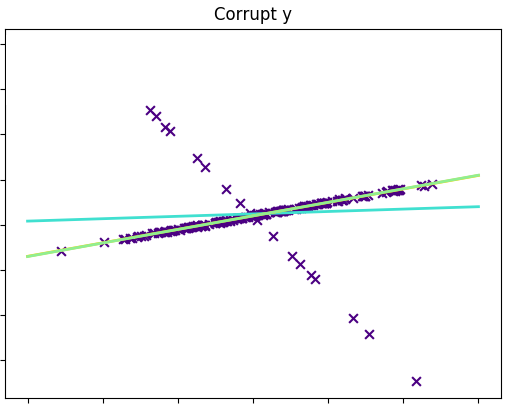
- Robust means solution is robust to outliers in the training set.
Weighted account for observations
Weighted account for observation
Weighted account for observations $$ \sum_{n=1}^{N}w_{n}(x_{n}^{T}\beta-y_{n})^{2} $$
- Weights may be:
- increased for incorrectly predicted objects
- algorithm becomes more oriented on error correction
- decreased for incorrectly predicted objects
- they may be considered outliers that break our model
Solution for weighted regression
$$ \sum_{n=1}^{N}w_{n}\left(x_{n}^{T}\beta-y_{n}\right)^{2}\to\min_{\beta\in\mathbb{R}} $$Stationarity condition: $$ \sum_{n=1}^{N}w_{n}x_{n}^{d}\left(x_{n}^{T}\beta-y_{n}\right)=0 $$
Define $\{X\}_{n,d}=x_{n}^{d}$, $W=diag\{w_{1},...x_{N}\}$. Then
$$ X^{T}W\left(X\beta-y\right)=0 $$$$ \beta=\left(X^{T}WX\right)^{-1}X^{T}Wy $$Robust regression
Initialize $w_{1}=...=w_{N}=1/N$
Repeat:
- estimate regression $\widehat{y}(x)$ using observations $(x_{i},y_{i})$ with weights $w_{i}$.
- for each $i=1,2,...N$:
- calculate $\varepsilon_{i}=\widehat{y}(x_{i})-y_{i}$
- calculate $w_{i}=K\left(\left|\varepsilon_{i}\right|\right)$
- normalize weights $w_{i}=\frac{w_{i}}{\sum_{n=1}^{N}w_{n}}$
Comments: $K(\cdot)$ is some decreasing function, repetition may be
- predefined number of times
- until convergence of model parameters.
Example
Linear Classification (in general)
Analytical geometry reminder
Reminder
- $a=[a^{1},...a^{D}]^{T},\,b=[b^{1},...b^{D}]^{T}$
- Scalar product $\langle a,b\rangle=a^{T}b=\sum_{d=1}^{D}a_{d}b_{b}$
- $a\perp b$ means that $\langle a,b\rangle=0$
- Norm $\left\lVert a\right\rVert =\sqrt{\langle a,a\rangle}$
- Distance $\rho(a,b)=\left\lVert a-b\right\rVert =\sqrt{\langle a-b,a-b\rangle}$
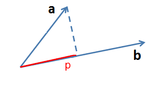
- $p=\langle a,\frac{b}{\left\lVert b\right\rVert }\rangle$
- $\left|p\right|=\left|\langle a,\frac{b}{\left\lVert b\right\rVert }\rangle\right|$- unsigned projection length
Orthogonal vector to hyperplane
Theorem 1
Vector $w$ is orthogonal to hyperplane $w^{T}x+w_{0}=0$
Proof: Consider arbitrary $x_{A},x_{B}\in\{x:\,w^{T}x+w_{0}=0\}$: $$ \begin{align} w^{T}x_{A}+w_{0}=0 \quad \text{ (1)}\\ w^{T}x_{B}+w_{0}=0 \quad \text{ (2)} \end{align} $$ By substracting (2) from (1), obtain $w^{T}(x_{A}-x_{B})=0$, so $w$ is orthogonal to hyperplane.
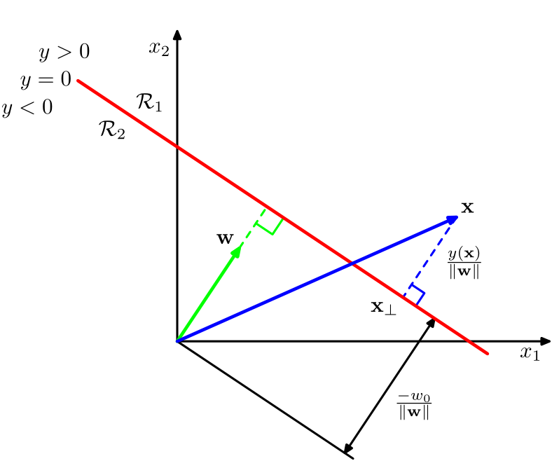
Distance from point to hyperplane
Theorem 2
Distance from point $x$ to hyperplane $w^{T}x+w_{0}=0$ is equal to $\frac{w^{T}x+w_{0}}{\left\lVert w\right\rVert }$.
Proof: Project $x$ on the hyperplane, let the projection be $p$ and complement $h=x-p$, orthogonal to hyperplane. Then $$ x=p+h $$
Since $p$ lies on the hyperplane, $$ w^{T}p+w_{0}=0 $$
Since $h$ is orthogonal to hyperplane and according to theorem 1 $$ h=r\frac{w}{\left\lVert w\right\rVert },\,r\in\mathbb{R}\text{ - distance to hyperplane}. $$
Distance from point to hyperplane
$$ x=p+r\frac{w}{\left\lVert w\right\rVert } $$After multiplication by $w$ and addition of $w_{0}$: $$ w^{T}x+w_{0}=w^{T}p+w_{0}+r\frac{w^{T}w}{\left\lVert w\right\rVert }=r\left\lVert w\right\rVert $$
because $w^{T}p+w_{0}=0$ and $\left\lVert w\right\rVert =\sqrt{w^{T}w}$. So we get, that $$ r=\frac{w^{T}x+w_{0}}{\left\lVert w\right\rVert } $$
Comments:
- From one side of hyperplane $r>0\Leftrightarrow w^{T}x+w_{0}>0$
- From the other side $r<0\Leftrightarrow w^{T}x+w_{0}<0$.
- Distance from hyperplane to origin 0 is $\frac{w_{0}}{\left\lVert w\right\rVert }$. So $w_{0}$ accounts for hyperplane offset.
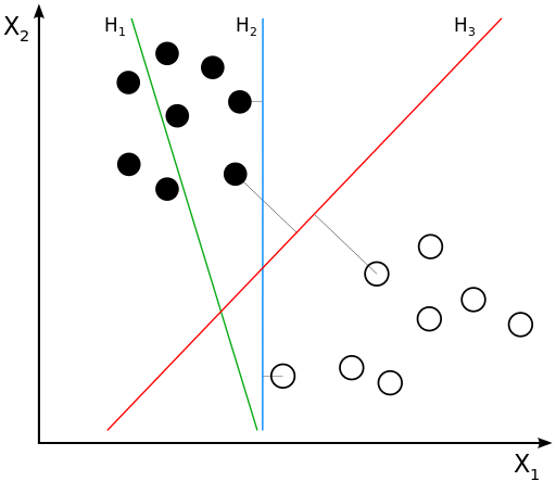
Binary linear classifier geometric interpretation
Binary linear classifier: $$ \widehat{y}(x)= sign\left(w^{T}x+w_{0}\right) $$
divides feature space by hyperplane $w^{T}x+w_{0}=0$.
- Confidence of decision is proportional to distance to hyperplane $\frac{\left|w^{T}x+w_{0}\right|}{\left\lVert w\right\rVert }$.
- $w^{T}x+w_{0}$ is the confidence that class is positive.
Consider the foolowing objects
| x1 | x2 |
|---|---|
| 0 | 1 |
| 1 | 0 |
| 1 | 1 |
| 2 | 2 |
| 2 | 3 |
| 3 | 2 |
Find class prediction if $(w_0 = -0.3 , w_1 = 0.1, w_2 = 0.1)$
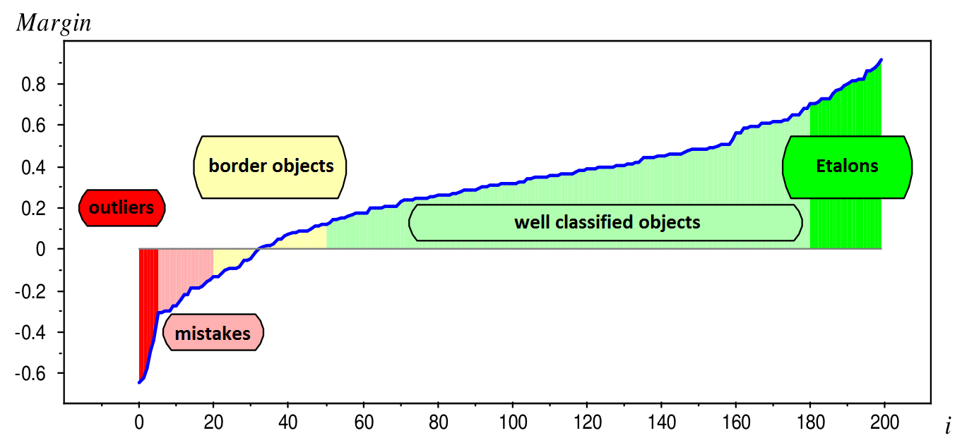
Margin of binary linear classifier
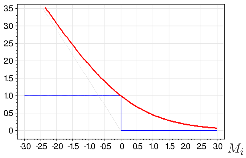
$$ M(x,y) =y\left(w^{T}x+w_{0}\right) $$- $ y \in \{-1,+1\}$
- Margin = score, how well classifier predicted true $y$ for object $x$.
- $M(x,y|w)>0$ <=> object $x$ is correctly classified as $y$
- signs of $w^{T}x+w_{0}$ and $y$ coincide
- $|M(x,y|w)|=\left|w^{T}x+w_{0}\right|$ - confidence of decision
- proportional to distance from $x$ to hyperplane $w^{T}x+w_{0}=0$.
Margin
Misclassification rate optimization
- Misclassification rate optimization: $$ \frac{1}{N}\sum_{n=1}^{N}\mathbb{I}[M(x_{n},y_{n}|w)<0]\to\min_{w} $$
is not recommended:
- discontinious function, can't use numerical optimization!
continous margin is more informative than binary error indicator.
If we select loss function $\mathcal{L}(M)$ such that $\mathbb{I}[M]\le\mathcal{L}(M)$ then we can optimize upper bound on misclassification rate: $$ \begin{gathered}\begin{gathered}\text{MISCLASSIFICATION RATE}\end{gathered} =\frac{1}{N}\sum_{n=1}^{N}\mathbb{I}[M(x_{n},y_{n}|w)<0]\\ \le\frac{1}{N}\sum_{n=1}^{N}\mathcal{L}(M(x_{n},y_{n}|w))=L(w) \end{gathered} $$
Weights optimization
- Margin = score, how well classifier predicted true $y$ for object $x$.
- Task: select such $w$ to increase $M(x_{n},y_{n}|w)$ for all $n$.
- Formalization: $$ \frac{1}{N}\sum_{n=1}^{N}\mathcal{L}\left(M(x_{n},y_{n}|w)\right)\to\min_{w} $$
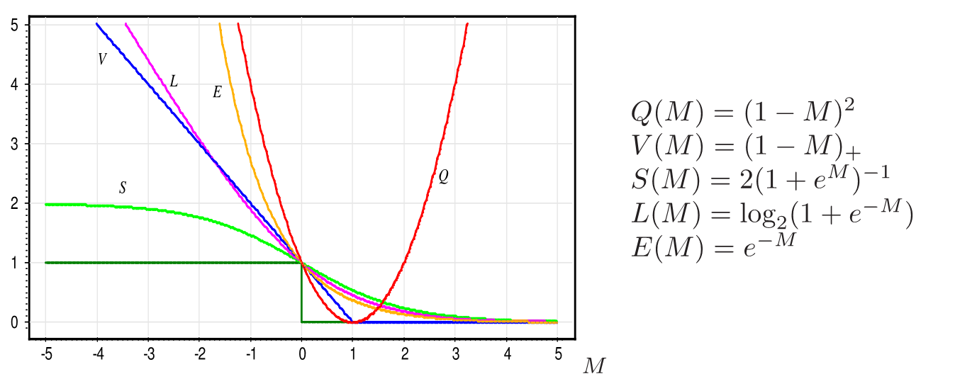
Common loss functions
Optimization
Same story as in linear regression
Regularization
Same story as in linear regression
$L_{1}$ regularization
$||w||_{1}$ regularizer should do feature selection.
Consider $$ L(w)=\sum_{n=1}^{N}\mathcal{L}\left(M(x_{n},y_{n}|w)\right)+\lambda\sum_{d=1}^{D}|w_{d}| $$
And gradient updates $$ \frac{\partial}{\partial w_{i}}L(w)=\sum_{n=1}^{N}\frac{\partial}{\partial w_{i}}\mathcal{L}\left(M(x_{n},y_{n}|w)\right)+\lambda sign (w_{i}) $$
$L_{2}$ regularization
$$ L(w)=\sum_{n=1}^{N}\mathcal{L}\left(M(x_{n},y_{n}|w)\right)+\lambda\sum_{d=1}^{D}w_{d}^{2} $$$$ \frac{\partial}{\partial w_{i}}L(w)=\sum_{n=1}^{N}\frac{\partial}{\partial w_{i}}\mathcal{L}\left(M(x_{n},y_{n}|w)\right)+2\lambda w_{i} $$$$ 2\lambda w_{i}\to0\text{ when }w_{i}\to0 $$- Strength of regularization $\to0$ as weights $\to0$.
- So $L_{2}$ regularization will not set weights exactly to 0.
Logistic Regression
Binary classification
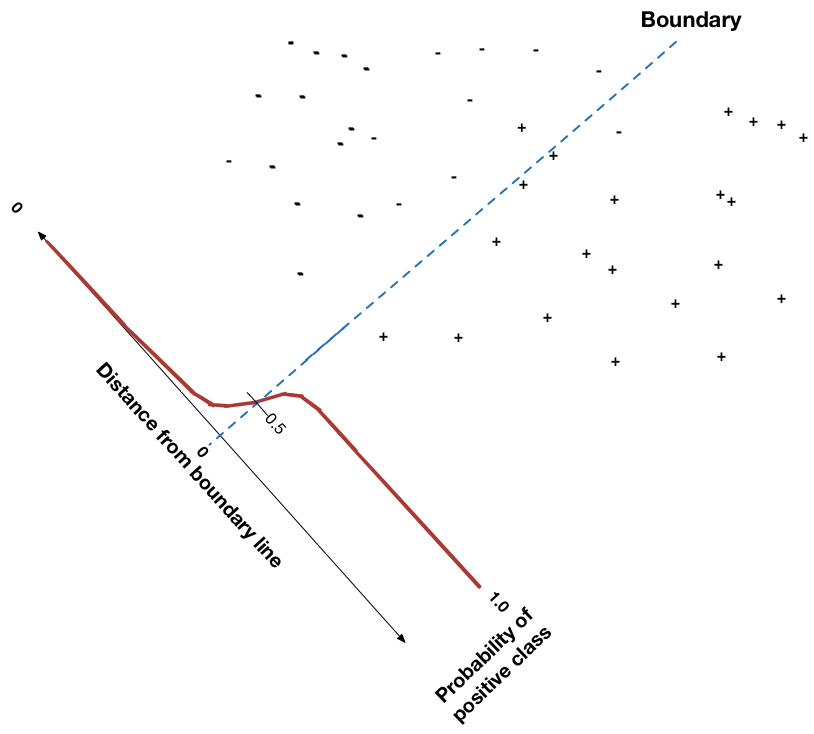
- Linear classifier: $$ score(\omega_{1}|x)=w^{T}x + w_0 = g(x) $$
- +relationship between score and class probability is assumed: $$ p(\omega_{1}|x)=\sigma(w^{T}x + w_0) $$
where $\sigma(z)=\frac{1}{1+e^{-z}}$ - sigmoid function
demo_sigmoid()
Binary classification: estimation
- Given our assumption:
- $p(y=+1|x)=\sigma(w^{T}x + w_0)$
- $p(y=-1|x)=1 - p(y=+1|x)$
we can write down Likelihood function: $$ \mathcal{L}(w) = \prod_{n=1}^N p(y_n=+1|x_n)^{\mathbb{I}[y_n = +1]} p(y_n=-1|x_n)^{\mathbb{I}[y_n = -1]} \rightarrow \max_w$$
Get rid if products: $$ -\ln{\mathcal{L}(w)} = - \sum_{n=1}^N \mathbb{I}[y_n = +1]\cdot\ln{\sigma(w^{T}x_n+w_0))} + \mathbb{I}[y_n = -1]\cdot\ln{(1-\sigma(w^{T}x_n+w_0))} \rightarrow \min_w$$ $$L(w) = -\ln{\mathcal{L}(w)} \rightarrow \min_w $$
Function $L(w)$ is also called log-loss
Another formulation
Using the property $1-\sigma(z)=\sigma(-z)$ obtain that $$ p(y=+1|x)=\sigma(w^{T}x+w_0)\Longrightarrow p(y=-1|x)=\sigma(-w^{T}x - w_0) $$
So for $y\in\{+1,-1\}$ $$ p(y|x)=\sigma(y(\langle w,x\rangle + w_0)) $$
Therefore ML estimation can be written as: $$ \prod_{n=1}^{N}\sigma( y_{n}(\langle w,x_{n}\rangle + w_0))\to\max_{w} $$
Loss function for 2-class logistic regression
For binary classification $p(y|x)=\sigma(y(\langle w,x\rangle + w_0))$
Estimation with ML:
$$ \prod_{n=1}^{N}\sigma(y_n(\langle w,x_n\rangle + w_0)) = \prod_{n=1}^{N}\sigma(y_n g(x_n)) = \to\max_{w} $$which is equivalent to $$ \sum_{n=1}^{N}\ln(1+e^{-y_ng(x_n)})\to\min_{w} $$
It follows that logistic regression is linear discriminant estimated with loss function $\mathcal{L}(M)=\ln(1+e^{-M})$.
Multiclass classification with binary classifiers
Multiclass classification with binary classifiers
- Task - make $C$-class classification using many binary classifiers.
Approaches:
one-versus-all
- for each $c=1,2,...C$ train binary classifier on all objects and output $\mathbb{I}[y_{n}=c]$,
- assign class, getting the highest score in resulting $C$ classifiers.
one-versus-one
- for each $i,j\in[1,2,...C],$ $i\ne j$ learn on objects with $y_{n}\in\{i,j\}$ with output $y_{n}$
- assign class, getting the highest score in resulting $C(C-1)/2$ classifiers.
Binary linear classifier
- For two classes $y\in\{+1,-1\}$ classifier becomes $$ \widehat{y}(x)=\begin{cases} +1, & w_{+1}^{T}x+w_{+1,0}>w_{-1}^{T}x+w_{-1,0}\\ -1 & \text{otherwise} \end{cases} $$
- This decision rule is equivalent to $$ \begin{align*} \widehat{y}(x) & =sign(w_{+1}^{T}x+w_{+1,0}-w_{-1}^{T}x+w_{-1,0})=\\ & =sign\left(\left(w_{+1}^{T}-w_{-1}^{T}\right)x+\left(w_{+1,0}-w_{-1,0}\right)\right)\\ & =sign\left(w^{T}x+w_{0}\right) \end{align*} $$ for $w=w_{+1}-w_{-1},\,w_{0}=w_{+1,0}-w_{-1,0}$.
- Decision boundary $w^{T}x+w_{0}=0$ is linear.
- Multiclass case can be solved using multiple binary classifiers with one-vs-all, one-vs-one
- can you imagine faulty situation with those approaches for linear classifiers?
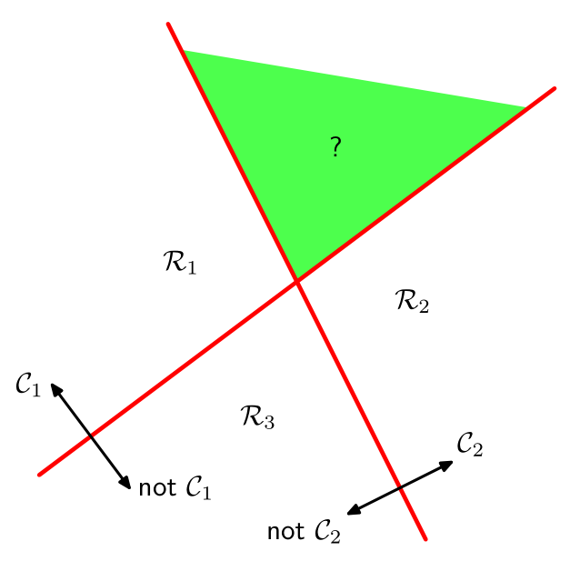
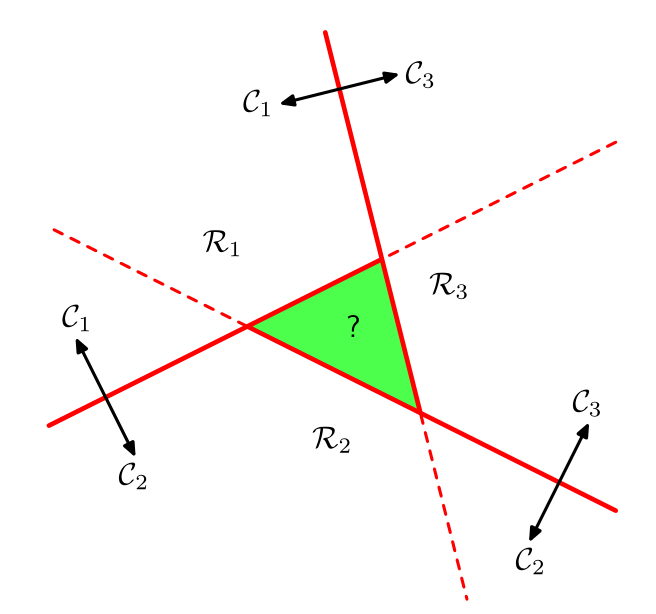
Linear classifier for multiple classes
- Classification among classes 1,2,...C.
- Use $C$ discriminant functions $g_{c}(x)=w_{c}^{T}x+w_{c0}$
- Decision rule: $$ \widehat{y}(x)=\arg\max_{c}g_{c}(x) $$
- Decision boundary between classes $y=i$ and $y=j$ is linear: $$ \left(w_{i}-w_{j}\right)^{T}x+\left(w_{i0}-w_{j0}\right)=0 $$
- Decision regions are convex
Logistic regression for multiple classes
Each class has a set of weights: $$ \begin{cases} score(\omega_{1}|x)=w_{1}^{T}x + w_{0,1} \\ score(\omega_{2}|x)=w_{2}^{T}x + w_{0,2}\\ \cdots\\ score(\omega_{C}|x)=w_{C}^{T}x + + w_{0,C} \end{cases} $$
+relationship between score and class probability is assumed:
$$ p(\omega_{c}|x)=softmax(\omega_c|W, x)=\frac{exp(w_{c}^{T}x + w_{0,c})}{\sum_{i}exp(w_{i}^{T}x + w_{0,i})} $$Estimation with ML: $$ \prod_{n=1}^{N}\prod_{c=1}^{C} softmax(\omega_c|W, x_n)^{\mathbb{I}[y_n = w_c]} $$
Which would lead us to cross-entropy loss function $$L(w) = - \sum_{n=1}^N\sum_{c=1}^{C} \mathbb{I}[y_n = w_c]\cdot\ln{\sigma(w_c^{T}x_n+w_{c,0}))}$$
Summary
- Linear classifier - classifier with linear discriminant functions.
- Binary linear classifier: $\widehat{y}(x)=sign(w^{T}x+w_{0})$.
- Perceptron, logistic, SVM - linear classifiers estimated with different loss functions.
- Weights are selected to minimize total loss on margins.
- Gradient descent iteratively optimizes $L(w)$ in the direction of maximum descent.
- Stochastic gradient descent approximates $\nabla_{w}L$ by averaging gradients over small subset of objects.
- Regularization gives smooth control over model complexity.
- $L_{1}$ regularization automatically selects features.