Data Analysis
Andrey Shestakov (avshestakov@hse.ru)
Feature Selection and Dimention Reduction. PCA.1
1. Some materials are taken from machine learning course of Victor Kitov
Feature Selection vs. Dimension Reduction
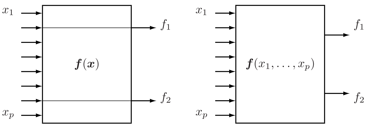
- Feature selection is a process of selecting a subset of original features with minimum loss of information related to final task (classification, regression, etc.)
- Dimension reduction is a result of some transformation of initial features to (possibly) lower dimension feature space
Why feature selection?
- increase predictive accuracy of classifier
- improve optimization stability by removing multicollinearity
- increase computational efficiency
- reduce cost of future data collection
- make classifier more interpretable
Not always necessary step
- some methods have implicit feature selection
Feature Selection Approaches
- Unsupervised methods
- don't use target feature
- Filter methdos
- use target feature
- consider each feature independently
- Wrapper methods
- uses model quality
- Embedded methdos
- embedded inside model
"Unsupervised" methods
- Determine feature importance regardless of target feature
- Your ideas?
Filter methods
- Features are considered independently of each other
- Individual predictive power is measures
Basically
- Order features with respect to feature importances $I(f)$: $$ I(f_{1})> I(f_{2})> \dots\ge I(f_{D}) $$
- Select top $m$ $$ \hat{F}=\{f_{1},f_{2},...f_{m}\} $$
- Simple to implement
- Usually quite fast
- When features are correlated, it will take many redundant features
Examples
- Correlation
- Which kind of relationship does correlation measure?
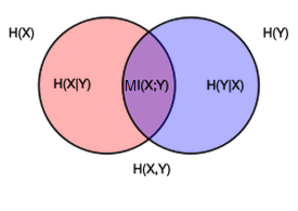
- Mutual Information
- Entropy of variable $Y$: $H(Y) = - \sum_y p(y)\ln p(y)$
- Conditional entropy of $Y$ after observing $X$: $H(y|x) = - \sum_x p(x) \sum_y p(y|x)\ln p(y|x) $
- Mutial information: $$MI(Y, X) = \sum_{x,y} p(x,y) \ln\left[\frac{p(x,y)}{p(x)p(y)}\right]$$
- Mutual information measures how much $X$ and $Y$ share information between each other
- $MI(Y,X) = H(Y) - H(Y|X)$
df_titanic = pd.read_csv('data/titanic.csv')
df_titanic.head()
P = pd.crosstab(df_titanic.Survived, df_titanic.Sex, normalize=True).values
print(P)
px = P.sum(axis=1)[:, np.newaxis]
py = P.sum(axis=0)[:, np.newaxis]
print(px)
print(py)
px.dot(py.T)
mutual_info(df_titanic.Sex, df_titanic.Survived)
Wrapper methods
- Selecting suboptimal subset of features
- Could be slow
- Examples:
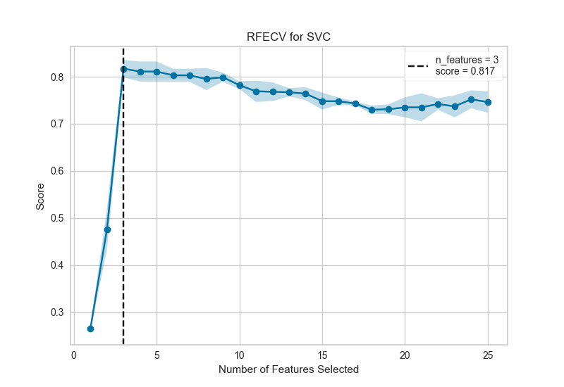
- Recursive Feature Elimination
- Consider full set of features
- Fit a model, measure feature importance (based on model)
- Remove least important feature(s)
- Repeat
- Boruta Algorithm
- Recursive Feature Elimination
Embedded methods
- Feature selection process in included in the model
- Examples:
- Decision Trees
- Linear model with L1 regularization
Feature Selection vs. Feature Extraction
PCA
- Intuition 2: Find a subspace $L$ (of lesser dimention) s.t. the sum of squares of differences between points and their projections is minimized
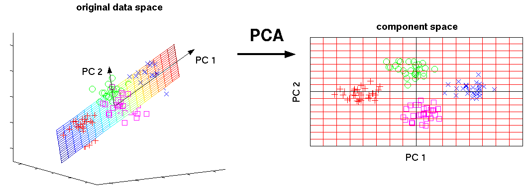
In other words, we can consider PCA as
- A transformation of your inital feature axes ...
- New axes are just a linear combination of initial axes
- New axes are orthogonal (orthonormal) to each other
- Variance of data across those axes is maximized
- ... which keeps only the most "informative" axes
How do we project data on new axes?
- Consider an object $x$ with 3 features: $x=(-0.343, -0.754, 0.241)$
- We can say that it is spanned on 3 basis vectors of our feature space: $$ e_1 = \left( \begin{array}{c} 1 \\ 0 \\ 0 \end{array} \right) \quad e_2 = \left( \begin{array}{c} 0 \\ 1 \\ 0 \end{array} \right) \quad e_3 = \left( \begin{array}{c} 0 \\ 0 \\ 1 \end{array} \right) \quad$$
- Consider new basis vectors:
- How do we project $x$ on it?
Projecting
$$ a_1 = \left( \begin{array}{c} -0.390 \\ 0.089 \\ -0.916 \end{array} \right) \quad a_2 = \left( \begin{array}{c} -0.639 \\ -0.742 \\ 0.200 \end{array} \right) \quad a_3 = \left( \begin{array}{c} -0.663 \\ 0.664 \\ 0.346 \end{array} \right) \quad$$$$ z = A^\top x = \left( \begin{array}{ccc} -0.390 & 0.089 & -0.916\\ -0.639 & -0.742 & 0.200 \\ -0.663 & 0.664 & 0.346 \end{array} \right) \left( \begin{array}{c} -0.343 \\ -0.754 \\ 0.241 \end{array} \right) = \left( \begin{array}{c} -1.154 \\ 0.828 \\ 0.190 \end{array} \right)$$That is: $$ z = -1.154 a_1 + 0.828 a_2 + 0.190 a_3$$
(Example from Mohammed J. Zaki, Ch7 )
- So how do we find those $a_i$?
- Orthonormality
- Maximize variance
- Vectors $a_i$ are called principal components
Construction of PCA
Construction of PCA
- Principal components $a_{1},a_{2},...a_{D}\in\mathbb{R}^{D}$ are orthonormal: $$\langle a_{i},a_{j}\rangle=\begin{cases} 1, & i=j\\ 0 & i\ne j \end{cases}$$
Maximize variance
- Datapoints in $X$ assumed to be centralized (and scaled)
- $z_i = a^\top x_i$ - projection of $x_i$ on $a$
- Variance across principal component $a$ for dataset $$ \begin{align} \sigma^2_a & = \frac{1}{n}\sum\limits_{i=1}^n(z_i - \mu_z)^2 \\ & = \frac{1}{n}\sum\limits_{i=1}^n(a^\top x_i)^2 \\ & = \frac{1}{n}\sum\limits_{i=1}^n a^\top( x_i x_i^\top) a \\ & = a^\top \left(\frac{1}{n}\sum\limits_{i=1}^n x_i x_i^\top \right) a \\ & = a^\top C a \rightarrow \\ & = a^\top X^\top X a \rightarrow \max_w \\ \end{align} $$
$C = X^\top X$ - convariance (correlation in case of scaled dataset) matrix
Construction of PCA
- $a_{1}$ is selected to maximize $a_1^\top X^\top X a_1$ subject to $\langle a_{1},a_{1}\rangle=1$
- $a_{2}$ is selected to maximize $a_2^\top X^\top X a_2$ subject to $\langle a_{2},a_{2}\rangle=1$, $\langle a_{2},a_{1}\rangle=0$
- $a_{3}$ is selected to maximize $a_3^\top X^\top X a_3$ subject to $\langle a_{3},a_{3}\rangle=1$, $\langle a_{3},a_{1}\rangle=\langle a_{3},a_{2}\rangle=0$
etc.
Derivation of 1st component
$$ \begin{equation} \begin{cases} a_1^\top X^\top X a_1 \rightarrow \max_{a_1} \\ a_1^\top a_1 = 1 \end{cases} \end{equation} $$- Lagrangian of optimization problem $$ \mathcal{L}(a_1, \nu) = a_1^\top X^\top X a_1 - \nu (a_1^\top a_1 - 1) \rightarrow max_{a_1, \nu}$$
- Derivative w.r.t. $a_1$ $$ \frac{\partial\mathcal{L}}{\partial a_1} = 2X^\top X a_1 - 2\nu a_1 = 0 $$
- so $a_1$ is selected from a set of eigenvectors of $X^\top X$. But which one?
Useful properties of $X^\top X$
- $X^\top X$ - symmetric and positive semi-definite
- $(X^\top X)^\top = X^\top X$
- $\forall w \in \mathbb{R}^D:\ w^\top (X^\top X) w \geq 0$
- Properties
- All eigenvalues $\lambda_i \in \mathbb{R}, \lambda_i \geq 0$ (we also assume $\lambda_1 \geq \lambda_2 \geq \dots \geq \lambda_d $)
- Eigenvectors for $\lambda_i \neq \lambda_j $ are orthogonal: $v_i^\top v_j = 0$
- For each unique eigenvalue $\lambda_i$ there is a unique $v_i$
Back to component 1
Initially, our objective was $$a_1^\top X^\top X a_1 \rightarrow \max_{a_1}$$
From lagrangian we derived that $$X^\top X a_1 = \nu a_1$$
Putting one in to another: $$ a_1^\top X^\top X a_1 = \nu a_1^\top a_1 = \nu \rightarrow \max$$
That means:
- $\nu$ should be the greatest eigenvalue of matrix $X^\top X$, which is $\lambda_1$
- $a_1$ is eigenvector, correspondent to $\lambda_1$
Derivation of 2nd component
$$ \begin{equation} \begin{cases} a_2^\top X^\top X a_2 \rightarrow \max_{a_2} \\ a_2^\top a_2 = 1 \\ a_2^\top a_1 = 0 \end{cases} \end{equation} $$- Lagrangian of optimization problem $$ \mathcal{L}(a_2, \nu,\alpha) = a_2^\top X^\top X a_2 - \nu (a_2^\top a_2 - 1) - \alpha (a_1^\top a_2) \rightarrow max_{a_2, \nu,\alpha}$$
- Derivative w.r.t. $a_2$ $$ \frac{\partial\mathcal{L}}{\partial a_2} = 2X^\top X a_2 - 2\nu a_2 - \alpha a_1 = 0 $$
Derivation of 2nd component
By multiplying by $a_1^\top$ : $$ a_1^\top\frac{\partial\mathcal{L}}{\partial a_2} = 2a_1^\top X^\top X a_2 - 2\nu a_1^\top a_2 - \alpha a_1^\top a_1 = 0 $$
It follows that $\alpha a_1^\top a_1 = \alpha = 0$, which means that $$ \frac{\partial\mathcal{L}}{\partial a_2} = 2X^\top X a_2 - \nu a_2 = 0 $$ And $a_2$ is selected from a set of eigenvectors of $X^\top X$. Again, which one?
Derivations of other components proceeds in the same manner
PCA algorithm
- Center (and scale) dataset
- Calculate covariance matrix $С=X^\top X$
- Find first $k$ eigenvalues and eigenvectors $$A = \left[ \begin{array}{cccc} \mid & \mid & & \mid\\ a_{1} & a_{2} & \ldots & a_{k} \\ \mid & \mid & & \mid \end{array} \right] $$
- Perform projection: $$ Z = XA $$
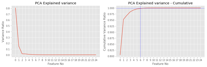
Explained variance or why do we neeed $\lambda$?
- As we remember $$a_i^\top X^\top X a_i = \lambda_i,$$ which means that $\lambda_i$ shows variance of data "explained" by $a_i$
- We can calculate explained variance ratio for $a_i$: $$ \frac{\lambda_{i}}{\sum_{d=1}^{D}\lambda_{d}} $$
(Supplementary) alternative view on PCA
Best hyperplane fit
For point $x$ and subspace $L$ denote:
- $p$: the projection of $x$ on $L$
- $h$: orthogonal complement
- $x=p+h$, $\langle p,h\rangle=0$,
Proposition
$\|x\|^2 = \|p\|^2 + \|h\|^2$
For training set $x_{1},x_{2},...x_{N}$ and subspace $L$ we can find:
- projections: $p_{1},p_{2},...p_{N}$
- orthogonal complements: $h_{1},h_{2},...h_{N}$.
Best subspace fit
Definition
Best-fit $k$-dimentional subspace for a set of points $x_1 \dots x_N$ is a subspace, spanned by $k$ vectors $v_1$, $v_2$, $\dots$, $v_k$, solving
$$ \sum_{n=1}^N \| h_n \| ^2 \rightarrow \min\limits_{v_1, v_2,\dots,v_k}$$or
$$ \sum_{n=1}^N \| p_n \| ^2 \rightarrow \max\limits_{v_1, v_2,\dots,v_k}$$Definition of PCA
Principal components $a_1, a_2, \dots, a_k$ are vectors, forming orthonormal basis in the k-dimentional subspace of best fit
Properties
- Not invariant to translation:
- center data before PCA: $$ x\leftarrow x-\mu\text{ where }\mu=\frac{1}{N}\sum_{n=1}^{N}x_{n} $$
- Not invariant to scaling:
- scale features to have unit variance before PCA
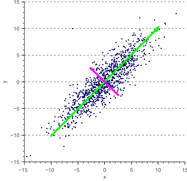
Example: line of best fit
- In PCA the sum of squared perpendicular distances to line is minimized:
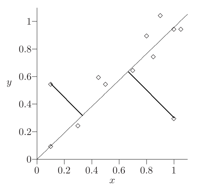
- What is the difference with least squares minimization in regression?
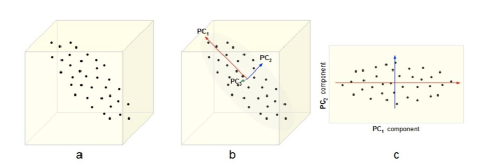
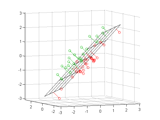
Example: plane of best fit
Construction of PCA
Construction of PCA
- Datapoints in $X$ assumed to be centralized and scaled (!)
- Principal components $a_{1},a_{2},...a_{D}\in\mathbb{R}^{D}$ are found such that $\langle a_{i},a_{j}\rangle=\begin{cases} 1, & i=j\\ 0 & i\ne j \end{cases}$
- $Xa_{i}$ is a vector of projections of all objects onto the $i$-th principal component.
- For any object $x$ its projections onto principal components are equal to: $$ p=A^{T}x=[\langle a_{1},x\rangle,...\langle a_{D},x\rangle]^{T} $$ where $A=[a_{1};a_{2};...a_{D}]\in\mathbb{R}^{DxD}$.
Construction of PCA
- $a_{1}$ is selected to maximize $\left\lVert Xa_{1}\right\rVert $ subject to $\langle a_{1},a_{1}\rangle=1$
- $a_{2}$ is selected to maximize $\left\lVert Xa_{2}\right\rVert $ subject to $\langle a_{2},a_{2}\rangle=1$, $\langle a_{2},a_{1}\rangle=0$
- $a_{3}$ is selected to maximize $\left\lVert Xa_{3}\right\rVert $ subject to $\langle a_{3},a_{3}\rangle=1$, $\langle a_{3},a_{1}\rangle=\langle a_{3},a_{2}\rangle=0$
etc.
PCA summary
- Dimensionality reduction - common preprocessing step for efficiency and numerical stability.
- Solution vectors $a_1,\dots,a_k$ are called top $k$ principal components.
- Principal component analysis - expression of $x$ in terms of first $k$ principal components.
- It is unsupervised linear dimensionality reduction.
- Solution is achieved on top $k$ eigenvectors $a_{1},...a_{k}$ of covariance matrix.
- PCA tutorial
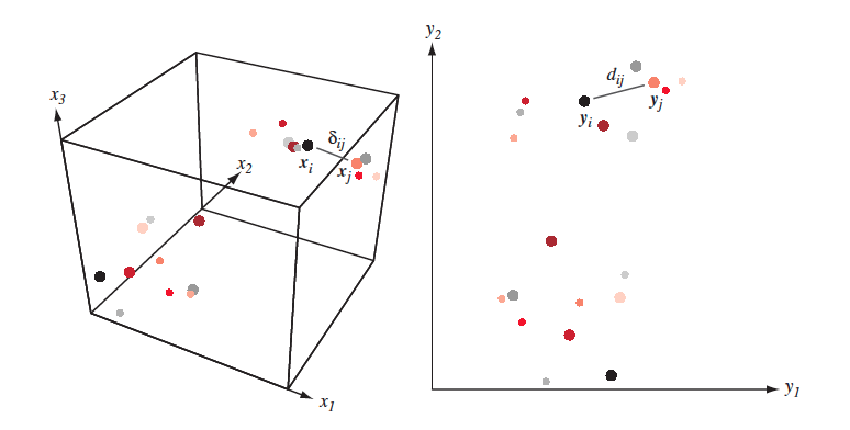
Multidimentional scaling - intuinition
Find feature space with lesser dimentions s.t. distances in initial space are conserved in the new one. A bit more formally:
- Given $X = [x_1,\dots, x_n]\in \mathbb{R}^{N \times D}$ and/or $\delta_{ij}$ - proximity measure between $(x_i,x_j)$ in initial feature space.
- Find $Y = [y_1,\dots,y_n] \in \mathbb{R}^{N \times d}$ such that $\delta_{ij} \approx d(y_i, y_j) = \|y_i-y_j\|^2$
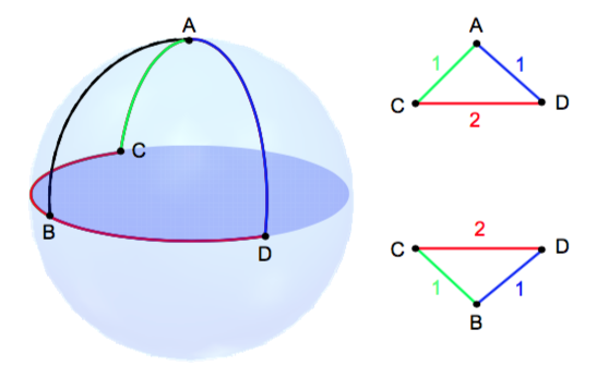
Multidimentional scaling
It is clear, that most of the times distances won't be conserved completely:
Multidimentional scaling approaches
- classical MDS (essentially PCA)
- metric MDS
- non-metric MDS
- But what if we want to conserve not the distances themselves, but the structure of inital dataset? Like neighbourhood of each point?
- Here comes t-SNE !!!
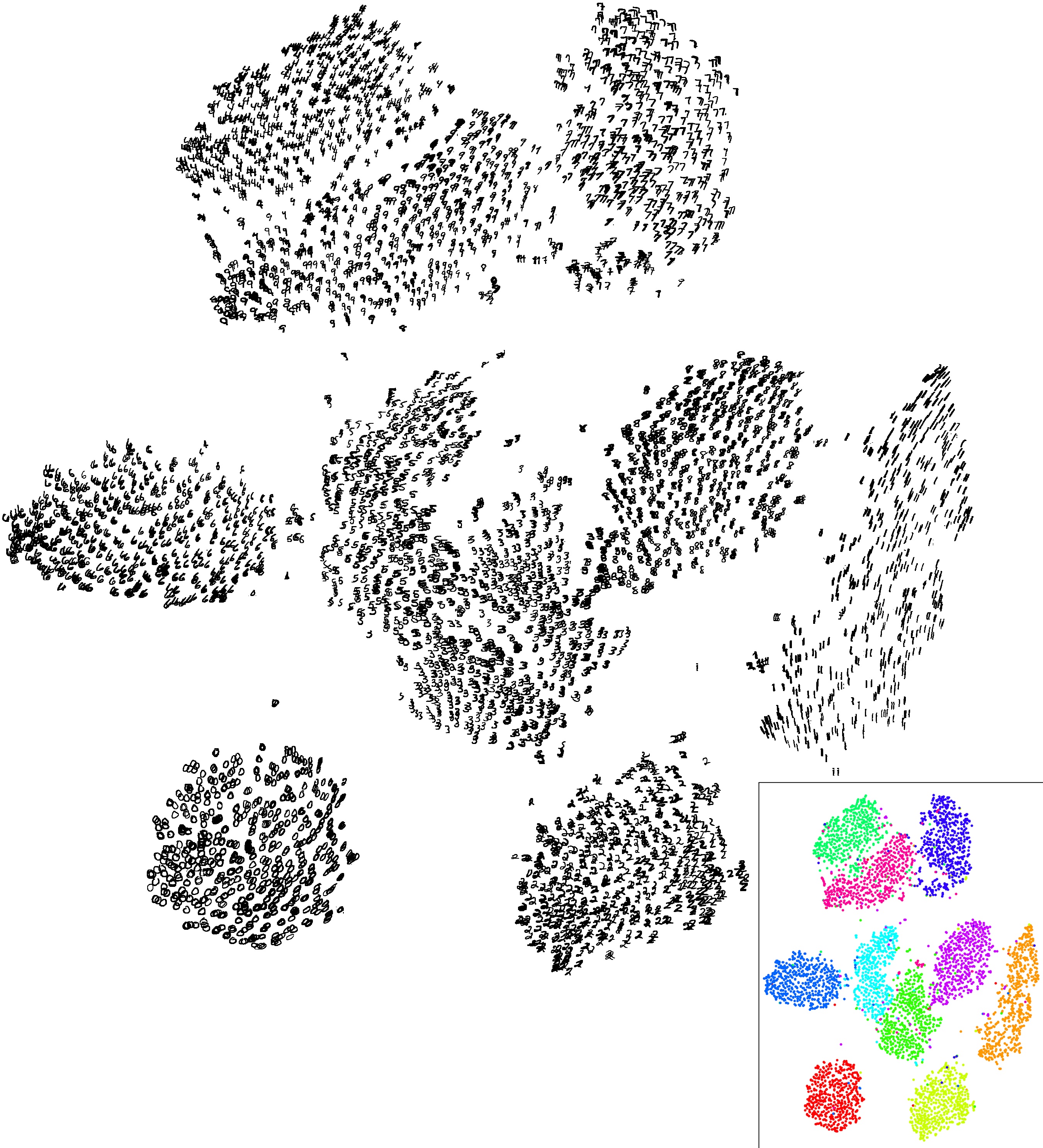
T-SNE
- t-SNE - is not multidimentional scaling, but the goal is somewhat similar
- There are going to be 3 types of similarities:
- Similarity between points in initial feature space
- Similarity between points in derived feature space
- Similarity between feature spaces!
T-SNE
- Similarity between points in initial feature space $\mathbb{R}^D$ $$ p(i, j) = \frac{p(i | j) + p(j | i)}{2N}, \quad p(j | i) = \frac{\exp(-\|\mathbf{x}_j-\mathbf{x}_i\|^2/{2 \sigma_i^2})}{\sum_{k \neq i}\exp(-\|\mathbf{x}_k-\mathbf{x}_i\|^2/{2 \sigma_i^2})} $$ $\sigma_i$ is set by user (implicitly)
- Similarity between points in derived feature space $\mathbb{R}^d, d << D$ $$ q(i, j) = \frac{g(|\mathbf{y}_i - \mathbf{y}_j|)}{\sum_{k \neq l} g(|\mathbf{y}_i - \mathbf{y}_j|)} $$ where $g(z) = \frac{1}{1 + z^2}$ - is student t-distribution with dof=$1$
- Similarity between feature spaces (Kullback–Leibler divergence) $$ J_{t-SNE}(y) = KL(P \| Q) = \sum_i \sum_j p(i, j) \log \frac{p(i, j)}{q(i, j)} \rightarrow \min\limits_{\mathbf{y}} $$
KL-Divergence
$$ KL(P \| Q) = \sum_z P(z) \log \frac{P(z)}{Q(z)} $$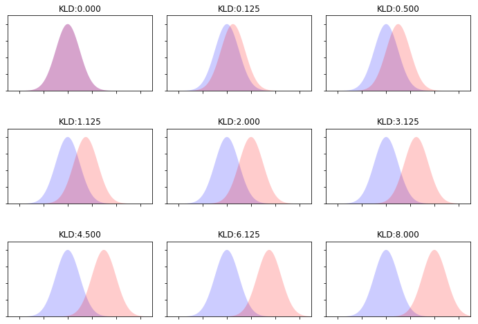
Optimization
- Optimize $J_{t-SNE}(y)$ with SGD
- Article
- Examples
- Demo and advises
- t-SNE is unstable
- Size of clusters means anything
- Distance means anything
- Random data can provide structure