Data Analysis
Andrey Shestakov (avshestakov@hse.ru)
Linear regression. Gradient-based optimization1
1. Some materials are taken from machine learning course of Victor Kitov
Let's recall previous lecture
- Decision trees
- Utilize the notion of impurity
- Work both for classification and regression
- Implicit feature selection
- good for features of different nature
- Parallel to axes class separating boundary
- Local greedy optimizaion
- Sensitive to even tiny data pertubations
Linear regression


Example: flat prices
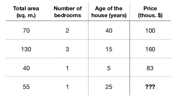
- Obviously, those characteristics somehow relate with price ($f: X \rightarrow Y$)
- Formalize a model to predict flat price: $$a(x) = a(total\_area, nmbr\_of\_bedrooms, house\_age) = \hat{y}$$
- Let it be a linear model: $$a(x) = \beta_0 + \beta_1\cdot total\_area + \beta_2 \cdot nmbr\_of\_bedrooms + \beta_3 \cdot house\_age$$
- Task - find coefficients $\beta_0,\dots, \beta_3$, that minimize loss function on training set
Cars price vs mileage
df_auto.plot(x='mileage', y='price', kind='scatter')

Linear regression
- Our goal - determine linear dependence between features $X$ and target vector $y$
- Define $x_n^d$ as $d$-th feature of $n$-th object, $y_{n} \in \mathbb{R}$ - target value for $n$-th object $$f(x_{n}, \beta) = \hat{y}_{n} = \beta_0 + \beta_1x_{n}^1 + \dots$$
- $x_{n}^0 = 1$ $\forall n$ - intercept
- Need to estimate $\beta_i$.
Ordinary Least Squares: $$ L(\beta_0,\beta_1,\dots) = \frac{1}{2N}\sum^{N}_{n=1}(\hat{y}_{n} - y_{n})^2 = \frac{1}{2N}\sum^{N}_{n=1}\left(\sum_{d=0}^{D}\beta_{d}x_{n}^{d}-y_{n}\right)^{2} \rightarrow \min\limits_{\beta} $$
Solution
Let's say $f(x, \beta) = \beta_0 + \beta_1x_1$
$$L(\beta_0, \beta_1) = \dots$$What do we do next?
Calculate partial derivatives wrt $\beta_0$, $\beta_1$ and set them to $0$:
$$ \frac{\partial L}{\partial \beta_0} = \frac{1}{N}\sum^{N}_{n=1}(\beta_0 + \beta_1x_{n}^1 - y_{n}) = 0$$$$ \frac{\partial L}{\partial \beta_1} = \frac{1}{N}\sum^{N}_{n=1}(\beta_0 + \beta_1x_{n}^1 - y_{n})x^1_{n} = 0$$Linear regression (in matrix form)
- Define $X\in\mathbb{R}^{NxD},\{X\}_{ij}$ defines the $j$-th feature of $i$-th object, $y\in\mathbb{R}^{n}$ - vector with target values $$f(x, \beta) = \hat{y} = X\beta \quad \Leftrightarrow \quad \left( \begin{array}{c} \hat{y}_1 \\ \hat{y}_2 \\ \vdots \\ \hat{y}_n \end{array} \right) = \left( \begin{array}{ccccc} 1 & x_1^1 & x_1^2 & \cdots & x_1^d\\ 1 & x_2^1 & x_2^2 & \cdots & x_2^d\\ \cdots & \cdots & \cdots & \cdots & \cdots\\ 1 & x_n^1 & x_n^2 & \cdots & x_n^d\end{array} \right) \cdot \left( \begin{array}{c} \beta_0 \\ \beta_1 \\ \vdots\\ \beta_d \end{array} \right) $$
- Need to estimate $\beta_i$.
Ordinary Lears Squares: $$ L(\beta) = \frac{1}{2N}(\hat{y} - y)^{\top}(\hat{y} - y) = \frac{1}{2N}(X\beta - y)^{\top}(X\beta - y) \rightarrow \min\limits_{\beta} $$
Solution (in matrix form)
Expand a bit $$ \begin{align*} L(\beta) & = \frac{1}{2N}(X\beta - y)^{\top}(X\beta - y) \\ & = \frac{1}{2N}\left( \beta^\top X^\top X \beta - 2 (X\beta)^\top y + y^\top y \right) \end{align*} $$
Calculate vector of partial derivatives - gradient
Some reminders
$$\begin{array}{rcl} \frac{\partial}{\partial x} x^T a &=& a \\ \frac{\partial}{\partial x} x^T A x &=& \left(A + A^T\right)x \\ \frac{\partial}{\partial A} x^T A y &=& xy^T \end{array}$$Comments
- This is the global minimum, because the optimized criteria is convex.
- Geometric interpretation:
- find linear combination of feature measurements that best reproduce $y$
- solution - combinaton of features, giving projection of $y$ on linear span of feature measurements.
- Why using Normal Equation could be bad?
- Calculating inverse costs a lot
- Not all matrices have it (singular matrices)
Linearly dependent features (multicollinearity)
- Solution $\widehat{\beta}=(X^{T}X)^{-1}X^{T}y$ exists when $X^{T}X$ is non-singular
- Problem occurs when one of the features is a linear combination of the other(s) (linear dependency)
- interpretation: non-identifiability of $\widehat{\beta}$ for linearly dependent features:
- linear dependence: $\exists\alpha:\,x^{T}\alpha=0\,\forall x$
- suppose $\beta$ solves linear regression $y=x^{T}\beta$
- then $x^{T}\beta\equiv x^{T}\beta+kx^{T}\alpha\equiv x^{T}(\beta+k\alpha)$, so $\beta+k\alpha$ is also a solution!
- interpretation: non-identifiability of $\widehat{\beta}$ for linearly dependent features:
- Multicollinearity can be exact and not exact, which is also bad
Examples of linear dependency
- $x$ miles $\approx 1.6\cdot x$ kms
- total flat area $\approx$ area of living rooms $+$ area of kitchen
- dummy variable trap!
df_auto.plot(x='mileage', y='price', kind='scatter')
df_auto.loc[:, ['mileage', 'price']].head()
X_train = df_auto.mileage.values.reshape(-1, 1)
y_train = df_auto.price.values

model = LinearRegression()
model.fit(X_train, y_train)

print('Модель:\nprice = %.2f + (%.2f)*mileage' % (model.intercept_, model.coef_[0]))

y_hat = model.predict(X_train)

df_auto.plot(x='mileage', y='price', kind='scatter')
_ = plt.plot(X_train, y_hat, c='r')

df_auto = df_auto.assign(kilometrage = lambda r: r.mileage*1.6)
df_auto.loc[:, ['mileage', 'kilometrage', 'price']].head()
X_train = df_auto.loc[:, ['mileage', 'kilometrage']].values
y_train = df_auto.price.values

model = LinearRegression()
model.fit(X_train, y_train)

print('Модель:\nprice = %.2f + (%.2f)*mileage + (%.2f)*kilometrage' % (model.intercept_, model.coef_[0], model.coef_[1],))

y_hat = model.predict(X_train)

df_auto.plot(x='mileage', y='price', kind='scatter')
_ = plt.plot(X_train[:, 0], y_hat, c='r')

Linearly dependent features
- Problem may be solved by:
- feature selection
- dimensionality reduction
- imposing additional requirements on the solution (regularization)
Analysis of linear regression
Advantages:
- single optimum, which is global (for non-singular matrix)
- analytical solution
- interpretable solution and algorithm
Drawbacks:
- too simple model assumptions (may not be satisfied)
- $X^{T}X$ should be non-degenerate (and well-conditioned)
Intuition
$$ L(\beta_0, \beta_1) = \frac{1}{2N}\sum_{n=1}^N(\beta_0 + \beta_1x^1_{n} - y_{n})^2$$- Suppose we have some initial approximation of $(\hat{\beta_0}, \hat{\beta_1})$
- How should we change it in order to improve?
sq_loss_demo()

Tiny Refresher
Derivative of $f(x)$ in $x_0$: $$ f'(x_0) = \lim\limits_{h \rightarrow 0}\frac{f(x_0+h) - f(x_0)}{h}$$
Derivative shows the slope of tangent line in $x_0$
- If $x_0$ is extreme point of $f(x)$ and $f'(x_0)$ exists $\Rightarrow$ $f'(x_0) = 0$
interact(deriv_demo, h=FloatSlider(min=0.0001, max=2, step=0.005), x0=FloatSlider(min=1, max=15, step=.2))
Tiny Refresher
- In multidimential world we switch to gradients and directional derivatives: $$ f'_v(x_0) = \lim\limits_{h \rightarrow 0}\frac{f(x_0+hv) - f(x_0)}{h} = \frac{d}{dh}f(x_{0,1} + hv_1, \dots, x_{0,d} + hv_d) \rvert_{h=0}, \quad ||v|| = 1 \quad \text{directional derivatives}$$
Tiny Refresher
- Unsing multivariate chain rule:
Tiny Refresher
$$ \langle \nabla f, v \rangle = || \nabla f || \cdot \cos{\phi}$$- Directional derivative is maximal when the direction is collinear to gradient
- gradient — direction of steepest ascent of $f(x)$
- antigradient — direction of steepest descent of $f(x)$
Given $L(\beta_0, \beta_1)$ calculate gradient (patial derivatives) $$ \frac{\partial L}{\partial \beta_0} = \frac{1}{N}\sum^{N}_{i=1}(\beta_0 + \beta_1x_{n}^1 - y^{n})$$ $$ \frac{\partial L}{\partial \beta_1} = \frac{1}{N}\sum^{N}_{i=1}(\beta_0 + \beta_1x_{n}^1 - y^{n})x^1_{n}$$
Or in matrix form: $$ \nabla_{\beta}L(\beta) = \frac{1}{N} X^\top(X\beta - y)$$
Run gradient update, which is simultaneous(!!!) update of $\beta$ in antigradient direction:
$$ \beta := \beta - \alpha\nabla_{\beta}L(\beta)$$- $\alpha$ - descent "speed"
Pseudocode
{python}
1.function gd(X, alpha, epsilon):

2.  initialise beta

3.  do:

4.      Beta = new_beta

5.      new_Beta = Beta - alpha*grad(X, beta)

6.  until dist(new_beta, beta) < epsilon

7. return betainteract(grad_demo, iters=IntSlider(min=0, max=20, step=1), alpha=FloatSlider(min=0.01, max=3, step=0.05))
Comments
- How do we set $\alpha$
- Feature scales matters

- Local minima*


Stochastic gradient descent
{python}
1.function sgd(X, alpha, epsilon):

2.  initialise beta

3.  do:

4.        X = shuffle(X)

5.        for x in X:

6.            Beta = new_beta

7.            new_Beta = Beta - alpha*grad(x, beta)

8.  until dist(new_beta, beta) < epsilon

9. return betastoch_grad_demo(iters=105, alpha=0.08)

Momentum
Idea: to move not only to current antigradient direction but consider previous one
$$ v_0 = 0$$$$ v_t = \gamma v_{t - 1} + \alpha\nabla_{\beta}{L(\beta)}$$$$ \beta = \beta - v_t$$where
- $\gamma$ — momentum term (usually 0.9)


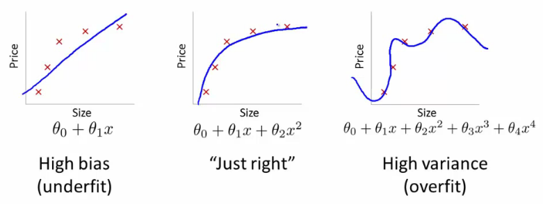
Nonlinear dependencies
Generalization by nonlinear transformations
Nonlinearity by $x$ in linear regression may be achieved by applying non-linear transformations to the features:
$$ x\to[\phi_{0}(x),\,\phi_{1}(x),\,\phi_{2}(x),\,...\,\phi_{M}(x)] $$$$ f(x)=\mathbf{\phi}(x)^{T}\beta=\sum_{m=0}^{M}\beta_{m}\phi_{m}(x) $$The model remains to be linear in $\beta$, so all advantages of linear regression remain.
Typical transformations
- $x^{i}\in[a,b]$ : binarization of feature
- $x^{i}x^{j}$ : interaction of features
- $\exp\left\{ -\gamma\left\lVert x-\tilde{x}\right\rVert ^{2}\right\} $ : closeness to reference point $\tilde{x}$
- $\ln x_{k}$ : the alignment of the distribution with heavy tails
demo_weights()

Regularization & restrictions
Intuition
 , width=800
Regularization
- Regularization - technique that reduces model complexity to prevent overfitting
- Desired outcomes:
- train loss goes up
- test loass goes down
- Have we already seen it?
Regularization
- Insert additional requirement for regularizer $R(\beta)$ to be small: $$ \sum_{n=1}^{N}\left(x_{n}^{T}\beta-y_{n}\right)^{2}+\lambda R(\beta)\to\min_{\beta} $$
- $\lambda>0$ - hyperparameter.
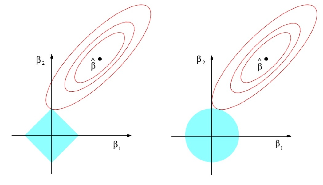
- $R(\beta)$ penalizes complexity of models. $$ \begin{array}{ll} R(\beta)=||\beta||_{1} & \mbox{Lasso regression}\\ R(\beta)=||\beta||_{2}^{2} & \text{Ridge regression} \end{array} $$
- Not only accuracy matters for the solution but also model simplicity!
- $\lambda$ controls complexity of the model:$\uparrow\lambda\Leftrightarrow\text{complexity}$$\downarrow$.
Comments
Dependency of $\beta$ from $\lambda$ for ridge (A) and LASSO (B):
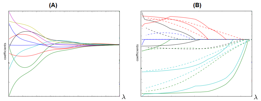
LASSO can be used for automatic feature selection.
- $\lambda$ is usually found using cross-validation on exponential grid, e.g. $[10^{-6},10^{-5},...10^{5},10^{6}]$.
- It's always recommended to use regularization because
- it gives smooth control over model complexity.
- reduces ambiguity for multiple solutions case.
df_auto.loc[:, ['mileage', 'kilometrage', 'price']].head()
X_train = df_auto.loc[:, ['mileage', 'kilometrage']].values
y_train = df_auto.price.values

model = Lasso()
# model = Ridge()
model.fit(X_train, y_train)

print('Модель:\nprice = %.2f + (%.2f)*mileage + (%.2f)*kilometrage' % (model.intercept_, model.coef_[0], model.coef_[1],))

y_hat = model.predict(X_train)

df_auto.plot(x='mileage', y='price', kind='scatter')
_ = plt.plot(X_train[:, 0], y_hat, c='r')
ElasticNet
- ElasticNet:
$\alpha\in(0,1)$ - hyperparameter, controlling impact of each part.
- If two features $x^{i}$and $x^{j}$ are equal:
- LASSO may take only one of them
- Ridge will take both with equal weight
- but it doesn't remove useless features
- ElasticNet both removes useless features but gives equal weight for usefull equal features
- good, because feature equality may be due to chance on this particular training set
Ridge regression analytic solution
Ridge regression criterion $$ \sum_{n=1}^{N}\left(x_{n}^{T}\beta-y_{n}\right)^{2}+\lambda\beta^{T}\beta\to\min_{\beta} $$
Stationarity condition can be written as:
$$ \begin{gathered}2\sum_{n=1}^{N}x_{n}\left(x_{n}^{T}\beta-y_{n}\right)+2\lambda\beta=0\\ 2X^{T}(X\beta-y)+\lambda\beta=0\\ \left(X^{T}X+\lambda I\right)\beta=X^{T}y \end{gathered} $$so
$$ \widehat{\beta}=(X^{T}X+\lambda I)^{-1}X^{T}y $$Comments
- $X^{T}X+\lambda I$ is always non-degenerate as a sum of:
- non-negative definite $X^{T}X$
- positive definite $\lambda I$
- Intuition:
- out of all valid solutions select one giving simplest model
- Other regularizations also restrict the set of solutions.
Different account for different features
- Traditional approach regularizes all features uniformly: $$ \sum_{n=1}^{N}\left(x_{n}^{T}\beta-y_{n}\right)^{2}+\lambda R(\beta)\to\min_{w} $$
- Suppose we have $K$ groups of features with indices: $$ I_{1},I_{2},...I_{K} $$
- We may control the impact of each group on the model by: $$ \sum_{n=1}^{N}\left(x_{n}^{T}\beta-y_{n}\right)^{2}+\lambda_{1}R(\{\beta_{i}|i\in I_{1}\})+...+\lambda_{K}R(\{\beta_{i}|i\in I_{K}\})\to\min_{w} $$
- $\lambda_{1},\lambda_{2},...\lambda_{K}$ can be set using cross-validation
- In practice use common regularizer but with different feature scaling.
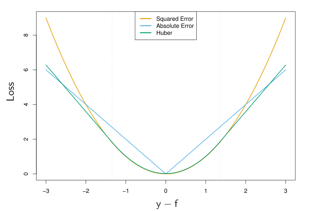
Different loss-functions
Idea
- Generalize squared to arbitrary loss: $$ \sum_{n=1}^{N}\left(x^{T}\beta-y_{n}\right)^{2}\to\min_{\beta}\qquad\Longrightarrow\qquad\sum_{n=1}^{N}\mathcal{L}(x_{n}^{T}\beta-y_{n})\to\min_{\beta} $$
- Robust means solution is robust to outliers in the training set.
References
- Elements of Statistical Learning (Trevor Hastie, Robert Tibshirani, Jerome Friedman) - Chapter 3