Data Analysis

Andrey Shestakov (avshestakov@hse.ru)

---

Supervised learning quality measures¹

^{1. Some materials are taken from machine learning course of Victor Kitov}

%matplotlib inline

import pandas as pd
import numpy as np
import matplotlib.pyplot as plt

plt.style.use('seaborn-talk')
plt.rcParams['figure.figsize'] = (15,10)

# Для кириллицы на графиках
font = {'family': 'Verdana',
        'weight': 'normal'}
plt.rc('font', **font)

from ipywidgets import interact, IntSlider, fixed, FloatSlider
    
import warnings
warnings.filterwarnings('ignore')

Let's recall previous lecture

• Linear Classification
  • Binary linear classifier: $g(x) = w^{T}x+w_{0}$
  • Classification $\widehat{y}(x)=sign(w^{T}x+w_{0})$
  • Various multiclassification approaches: 1-vs-all, 1-vs-1, etc..
• Perceptron, logistic, SVM - linear classifiers estimated with different loss functions
• Loss function for logistic regression is log-loss
  • $L(g(x), y) = \sum_{n=1}^{N}\ln(1+e^{-y_ng(x_n)})\to\min_{w}$
• Optimized with gradient descent

Model Selection

Model Selection

• If we have several models we need to understand which one is better then the other

• Check if ML model is performed better then simple heuristics or (almost) zero-information prediction, or simple baseline models
  • Always predict the majority class (classification)
  • Always predict the mean value (regression)
  • Build a simple model and compare its performance with your sophisticated model

• If performance of complex model is similar to performance of more simplistic model use the latter!

• Understand the profit of our model in business domain (see this)

Before we go

Recall the difference between loss function and quality measures

• Loss functions are directly optimized by algorithms
• Loss functions allways can be computed for a single object
• Quality measures are usually computed for a set of objects

Quality measures: Regression

1. (R)MSE ((Root) Mean Squared Error)

$$ L(\hat{y}, y) = \frac{1}{N}\sum\limits_{n=1}^N (y_n - \hat{y}_n)^2$$

2. MAE (Mean Absolute Error)

$$ L(\hat{y}, y) = \frac{1}{N}\sum\limits_{n=1}^N |y_n - \hat{y}_n|$$

• What are key differences?
• What are key issues?

MAE and MSE

• Different scales
• MSE penalize greater error more

• MAE is robust to outliers

  

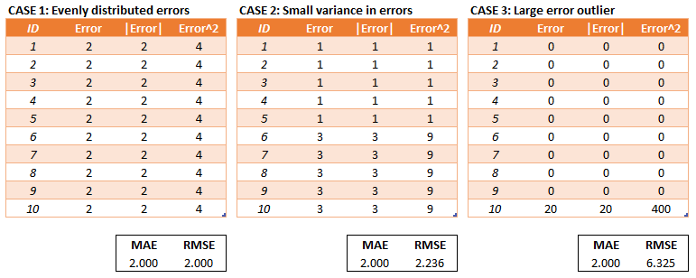
• We can compare models with MAE and MSE but it is hard to tell if a model is good overall...

3. RSE (Relative Squared Error)

$$ L(\hat{y}, y) = \sqrt\frac{\sum\limits_{n=1}^N (y_n - \hat{y}_n)^2}{\sum\limits_{n=1}^N (y_n - \bar{y})^2}$$

4. RAE (Relative Absolute Error)

$$ L(\hat{y}, y) = \frac{\sum\limits_{n=1}^N |y_n - \hat{y}_n|}{\sum\limits_{n=1}^N |y_n - \bar{y}|}$$

5. MAPE (Mean Absolute Persentage Error)

$$ L(\hat{y}, y) = \frac{100}{N} \sum\limits_{n=1}^N\left|\frac{ y_n - \hat{y}_n}{y_n}\right|$$

6. RMSLE (Root Mean Squared Logarithmic Error)

$$ L(\hat{y}, y) = \sqrt{\frac{1}{N}\sum\limits_{n=1}^N(\log(y_n + 1) - \log(\hat{y}_n + 1))^2}$$

• what is so special about it?

y = 10000
y_hat = np.linspace(0, 30000, 151)
# log error
error1 = np.sqrt((np.log(y+1) - np.log(y_hat + 1))**2)

# squared error
error2 = (y - y_hat)**2 /1000.

plt.plot(y_hat, error1, label='RMSLE'); plt.plot(y_hat, error2, label='MSE'); plt.xlabel('$\hat{y}$'); plt.ylabel('Error')
plt.title('true value y = %.1f' % y); plt.legend(); plt.ylim(0, 10)

(0, 10)

More complex options: domain specific quality measures

Stock optimization task

• Some retail chain wants to optimize stock replenishments of different items
• For items we have characteristics like price, "best before" period, holding costs
• We want to build predictive model to forecast demand for each item and use it to put orders on our goods in the most optimal way

• What risks (potential losses) can retail chain meet?
• What real life factors can be considered in this case and how do we measure quality?

Quality measures: Classification

Confusion matrix

Confusion matrix $M=\{m_{ij}\}_{i,j=1}^{C}$ shows the number of $\omega_{i}$ class objects predicted as belonging to class $\omega_{j}$.

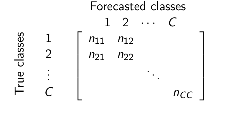
Diagonal elements correspond to correct classifications and off-diagonal elements - to incorrect classifications.

Confusion matrix

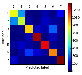
• We see here that errors are conсentrated between classes 1 and 2
• We can
  • unite classes 1 and 2 into class "1+2"
  • solve 6-class classification problem (instead of 7)
  • try to separate classes 1 and 2 afterwards

2 classes case

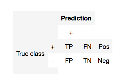
• TP (true positive) - currectly predicted positives
• FP (false positive) - incorrectly predicted negatives (1st order error)
• FN (false negative) - incorrectly predicted positives (2nd order error)
• TN (true negative) - currectly predicted negatives
• Pos (Neg) - total number of positives (negatives)

• Provide examples of task with positive classes and negative classes

• Why do you define them in that way and not another?

2 classes case

• $ \text{accuracy} = \frac{TP + TN}{Pos+Neg}$
• $ \text{error rate} = 1 -\text{accuracy}$
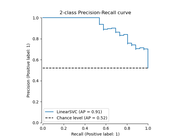
• $ \text{precision} =\frac{TP}{TP + FP}$ - (точность)
  • Ratio of objects marked positive are actually positive
• $ \text{recall} =\frac{TP}{TP + FN} = \frac{TP}{Pos}$ - (полнота)
  • Ratio of positive objects currectly classified
• $ \text{F}_\beta \text{-score} = (1 + \beta^2) \cdot \frac{\mathrm{precision} \cdot \mathrm{recall}}{(\beta^2 \cdot \mathrm{precision}) + \mathrm{recall}}$
  • why harmonic mean?

• What about multiclassification case?

from mpl_toolkits.mplot3d import Axes3D


def demo_fscore(beta=1):
    
    fig = plt.figure()
    ax = fig.gca(projection='3d')
    
    prec = np.linspace(0, 1, 100)
    rec = np.linspace(0, 1, 100)
    
    P, R = np.meshgrid(prec, rec)
    
    F = (1 + beta**2) * (P*R)/((beta**2 * P) + R)
    
    # Plot the surface.
    surf = ax.plot_surface(P, R, F, cmap=plt.cm.coolwarm, alpha=0.3,
                               linewidth=0, antialiased=False)

    # Customize the z axis.
    ax.set_zlim(-0.01, 1.01)
    
    ax.view_init(30,200)
    ax.set_xlabel('precision')
    ax.set_ylabel('recall')
    ax.set_zlabel('F-score')
    ax.set_title('beta = %.2f'%beta)

    # Add a color bar which maps values to colors.
    fig.colorbar(surf)
    plt.show()
    
   

fig = interact(demo_fscore, beta=FloatSlider(min=0.1, max=5, step=0.2, value=1))

Discriminant decision rules

• Decision rule based on discriminant functions:

  • predict $\omega_{1}$ $\Longleftrightarrow$ $g_{1}(x)-g_{2}(x)>\mu$
  • predict $\omega_{1}$ $\Longleftrightarrow$ $g_{1}(x)/g_{2}(x)>\mu$ (for $g_{1}(x)>0,\,g_{2}(x)>0$)

• Decision rule based on probabilities:

  • predict $\omega_{1}$ $\Longleftrightarrow$$P(\omega_{1}|x)>\mu$

Class label versus class probability evaluation

• Discriminability quality measures evaluate class label prediction.
  • examples: error rate, precision, recall, etc..

• Reliability quality measures evaluate class probability prediction.
  • Example: probability likelihood: $$ \prod_{n=1}^{N}\widehat{p}(y_{n}|x_{n}) $$
  • Brier score: $$ \frac{1}{N}\sum_{n=1}^{N}\sum_{c=1}^{C}\left(\mathbb{I}[y_{n}=c]-\widehat{p}(y=c|x_{n})\right)^{2} $$
  • Logloss (cross entropy): $$ \frac{1}{N}\sum_{n=1}^{N}\sum_{c=1}^{C}\mathbb{I}[y_{n}=c]\ln(\widehat{p}(y=c|x_{n})) $$

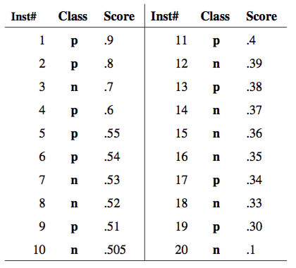
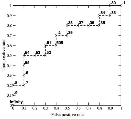
ROC curve

• ROC curve - is a function TPR(FPR).
• It shows how the probability of correct classification on positive classes ("recognition rate") changes with probability of incorrect classification on negative classes ("false alarm").
• It is build as a set of points TPR($\mu$), FPR($\mu$).

• If $\mu \downarrow$ , the algorithm predicts $\omega_{1}$ more often and

  • TPR=$1-\varepsilon_{1}$ $\uparrow$
  • FPR=$\varepsilon_{2}$ $\uparrow$

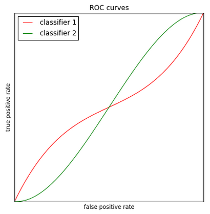
• Characterizes classification accuracy for different $\mu$.

  • more concave ROC curves are better

• $TPR = \frac{TP}{TP + FN}=\frac{TP}{Pos}$
• $FPR = \frac{FP}{FP + TN} = \frac{FP}{Neg}$

How to compare ROCs?

ROC-AUC

• Area under the ROC curve

• Global quality characteristic for different $\mu$

• AUC$\in[0,1]$

  • AUC = 0.5 - equivalent to random guessing
  • AUC = 1 - no errors classification.

• AUC property: it is equal to probability that for 2 random objects $x_{1}\in \text{"+"}$ and $x_{2}\in \text{"-"}$ it will hold that: $\widehat{p}(+|x_{1})>\widehat{p}(+|x_2)$

• What about unbalanced case?

Precision Recall Curve

• Build in the same manner as ROC curve
• Consider computing PR-AUC

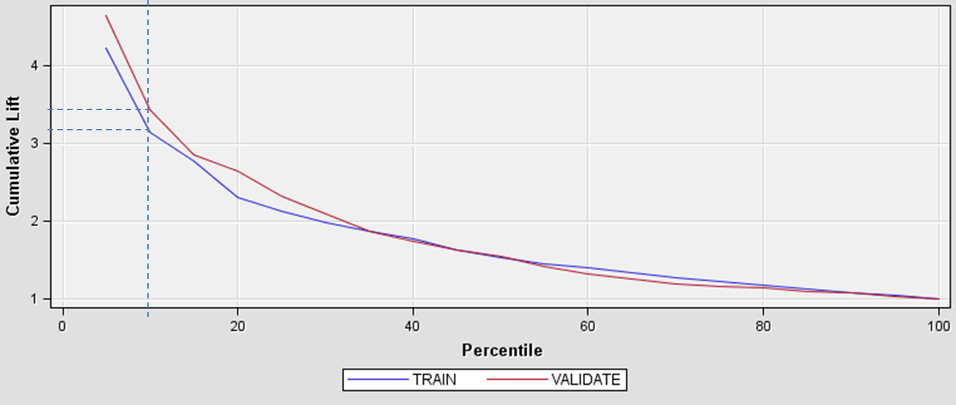
Model Lift

• Let $r_{POS}$ - positive class rate in the whole dataset

• Let $TPR @ K\%$ be positive class rate in top $K \%$ segment of the dateset, sorted by score

  $$ Model Lift @ K\% = \frac{TPR @ K\%}{r_{POS}} $$

Multiclassification averaging

• In multiclassification domain we can compute quality measures for each class in One-vs-All fasion
• Can we some how aggregate those values?
  • Micro-average
  • Macro-average
  • Weighted-average

Micro-average

• "Averaging over samples"

• For each class $c$ consider its confusion matrix

  
• Calculate $TP_c$, $TN_c$, $FP_c$, $FN_c$
• Calculate global measures as sum:
  • $TP = \sum_c TP_c$
  • $TN = \sum_c TN_c$
  • $FP = \sum_c FP_c$
  • $FN = \sum_c FN_c$
• Calculate final mesure (Recall, Presicion, etc) based on them

Macro-average

• "Averaging over classes"

• For each class $c$ consider its confusion matrix

  
• Calculate $TP_c$, $TN_c$, $FP_c$, $FN_c$
• Calculate measure (Recall, Presicion, etc) for each class individually
  • $\text{Recall}_c$
  • $\text{Presicion}_c$
  • $\text{F-score}_c$
• Calculate final mesure (Recall, Presicion, etc) as average

Weighted-average

• "Averaging over classes but with their representation rate"

• For each class $c$ consider its confusion matrix

  
• Calculate $TP_c$, $TN_c$, $FP_c$, $FN_c$
• Calculate measure (Recall, Presicion, etc) for each class individually
  • $\text{Recall}_c$
  • $\text{Presicion}_c$
  • $\text{F-score}_c$
• Calculate class weight as $w_c=\frac{|c|}{N}$
• Calculate final mesure (Recall, Presicion, etc) as weighted average

from sklearn import metrics

C="Coronavirus"
F="Flue"
O="Ok"

y_true = [C,C,C,C,C,C, F,F,F,F,F,F,F,F,F,F, O,O,O,O,O,O,O,O,O]
y_pred = [C,C,C,C,O,F, C,C,C,C,C,C,O,O,F,F, C,C,C,O,O,O,O,O,O]

print(metrics.confusion_matrix(y_true, y_pred))

print(metrics.classification_report(y_true, y_pred, digits=3))

[[4 1 1]
 [6 2 2]
 [3 0 6]]
              precision    recall  f1-score   support

 Coronavirus      0.308     0.667     0.421         6
        Flue      0.667     0.200     0.308        10
          Ok      0.667     0.667     0.667         9

    accuracy                          0.480        25
   macro avg      0.547     0.511     0.465        25
weighted avg      0.581     0.480     0.464        25

# Each column represents a class,
# Each row - an object
y_true = np.array([[0,1,0],
                   [0,1,1],
                   [1,0,1],
                   [0,0,1],
                   [0,0,0]])

y_pred = np.array([[0,1,1],
                   [0,1,1],
                   [0,1,0],
                   [0,0,0],
                   [1,0,1]])

print(metrics.classification_report(y_true, y_pred, digits=3))

              precision    recall  f1-score   support

           0      0.000     0.000     0.000         1
           1      0.667     1.000     0.800         2
           2      0.333     0.333     0.333         3

   micro avg      0.429     0.500     0.462         6
   macro avg      0.333     0.444     0.378         6
weighted avg      0.389     0.500     0.433         6
 samples avg      0.300     0.400     0.333         6

• Macro-averaging gives equal weight to each class
• Micro-averaging gives equal weight to each per-class classification decision
• Micro-averaging tends to over-emphasize the performance on the largest classes, while macro-averaging over-emphasizes the performance on the smallest

Useful links

• MAE vs MSE
• Intro to ROC Analysis
• Geometry of ROC Curve
• Illustrated Guide to ROC Curves
• ML meets ecomomics