Previously..
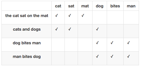
BoW text representation of documents
Each document $d_i$ from corpus $D$ is represented with vector $$ d_i = (w_1^i, w_2^i, \dots, w_N^i) $$
- $w_j^i$ - weight of word $j$ in document $i$
- word order is ignored
Problems with BoW
- Huge dimention of vectors (size of vocabulary)
- Problems with meaning capturing of individual words
- "Мера Левенштейна"
- "Расстояние Левенштейна"
- We want vector representation (embedding) of words s.t.:
- it is low-dimentional (128-1024)
- similar words have similar vectors
Distributional hypothesis
“You shall know a word by the company it keeps.” (J.R. Firth (1957))
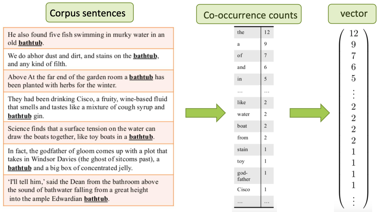
Approach 1: co-ocurence matrix
- Set some window size
- Calculate word-to-word co-ocurence counts $n_{uv}$
- or pointwise mutual information $PMI(u,v) = \log\left(\frac{p(u,v)}{p(u)\cdot p(v)}\right)$
Still, vectors are huge, so let's run dimention reduction!
Approach 1: co-ocurence matrix
Use truncated SVD!
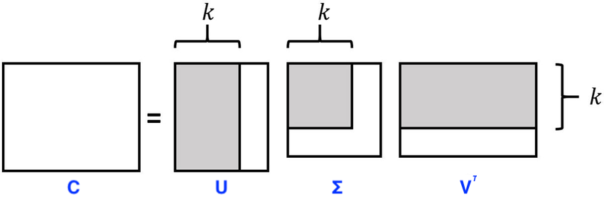
- Represent it as factorization of 2 matrices
- $\Phi = U\sqrt{\Sigma}$
- $\Theta = \sqrt{\Sigma}V$
- SVD provides us with the best approximation of $C$ in terms of Frobenius norm
- $L(C,\Phi,\Theta) = \sqrt{\sum_\limits{uv} \left(\phi_u^\top\theta_v - C_{uv}\right)^2}$
- get word embeddings as $\phi_u + \theta_u$
- Problems
- $C$ is mostly sparse
- Some co-occurences are quite common (for example with "the", "a" and other stopwords)
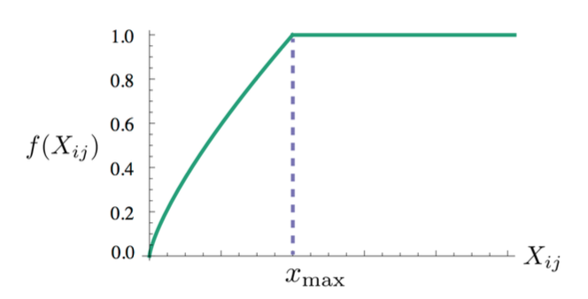
GloVe - GLObal VEctors (Pennington, et al. 2014)
- Introduces another loss function $$ L(W,\Phi,\Theta,b,c) = \frac{1}{2}\sum_\limits{uv}f(n_{uv})\cdot\left(\phi_u^\top\theta_v + b_u + c_v - \log(n_{uv})\right)^2 \rightarrow \min\limits_{\phi, \theta, b, c}$$
- Can be optimized via ALS (Alternating Least Squares)
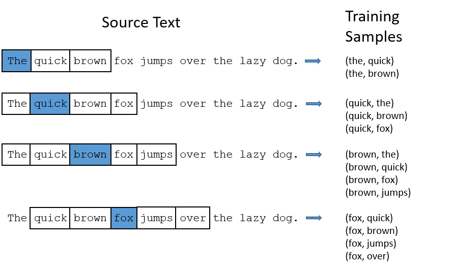
Approach 2: prediction of context
- Set some window size
- Go through each position $t$ in the text
- word on position $t$ is called center word $c$
- words within window frame from $c$ are called context words $o$
- Find such word vectors that maximized probability likelihood
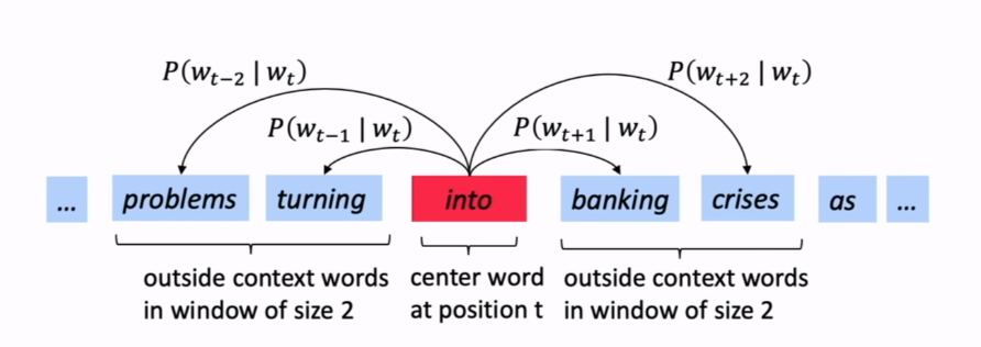
Approach 2: objective
$$ \begin{align*} L(\cdot) &= \prod_{t=1}^T\prod_{-m\leq j \leq m, j\neq0} p(w_{t+j} | w_t) \rightarrow \max \\ &\approx -\sum_{t=1}^T\sum_{-m\leq j \leq m, j\neq0} \log p(w_{t+j} | w_t) \rightarrow \min \end{align*} $$- How do we calculate $p(w_{t+j} | w_t)$?
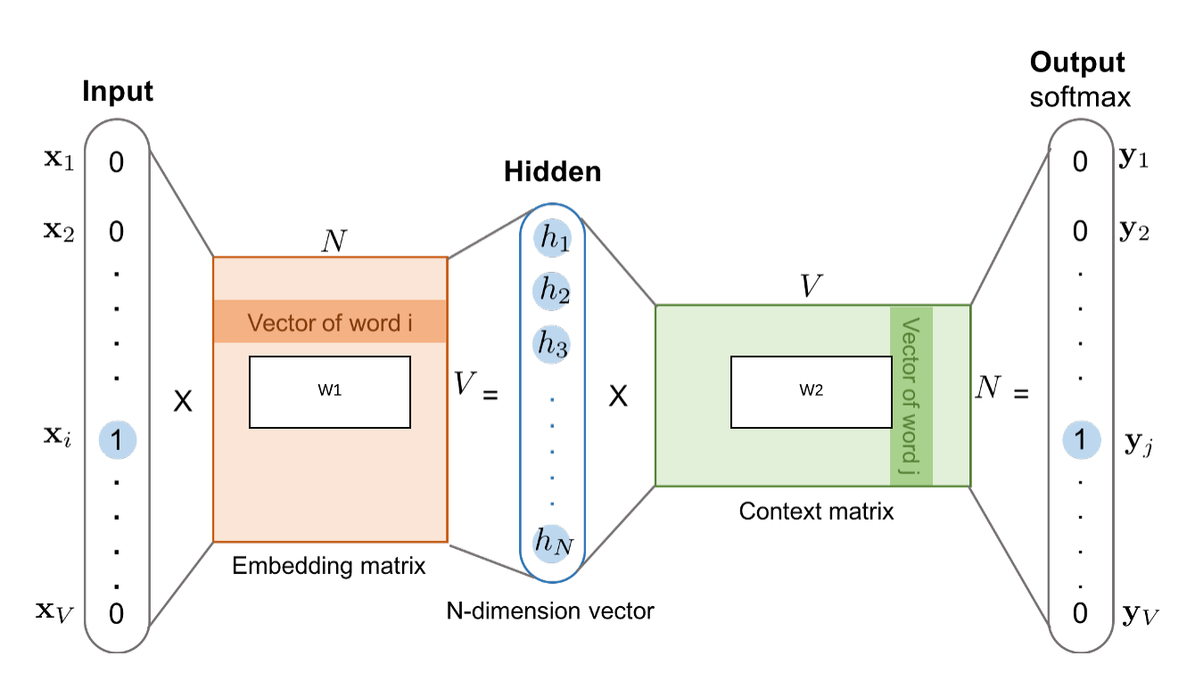
- Use the similarity of the word vectors for $c$ and $o$ to calculate the probability of $o$ given $c$ (or vice versa)
- Each word is having set of 2 vectors: $u$ when it is context word, $v$ when it is center word:
and our objective transformes to $$L(u,v) = -\sum_{(o,c)} \left(u_o^\top v_c - \log\left(\sum\limits_{w\in V} \exp(u_w^\top v_c)\right)\right) \rightarrow \min\limits_{u,v}$$
- Need to calculated last term more efficiently!
Negative sampling
- With given corpus we can mark pairs of words $(o,c)\in D$ as observed (positive class) ...
- and randomly generate unobserved pairs of words $(o`,c)\notin D$ (negative class)
Negative sampling
- similarly as it was for binary logistic regression: $$ p(o|c) = \sigma(u_o^\top v_c)$$
- Specifically, for each $(o, c) \in D$ we construct $k$ samples $(o_1, c ),\dots, (o_k, c)$, where each $o_j$ is drawn according to its unigram distribution to the power $3/4$
- Need to compute gradient updates for $u_o$, $v_c$ and $u_{o`}$
Skip-Gram model

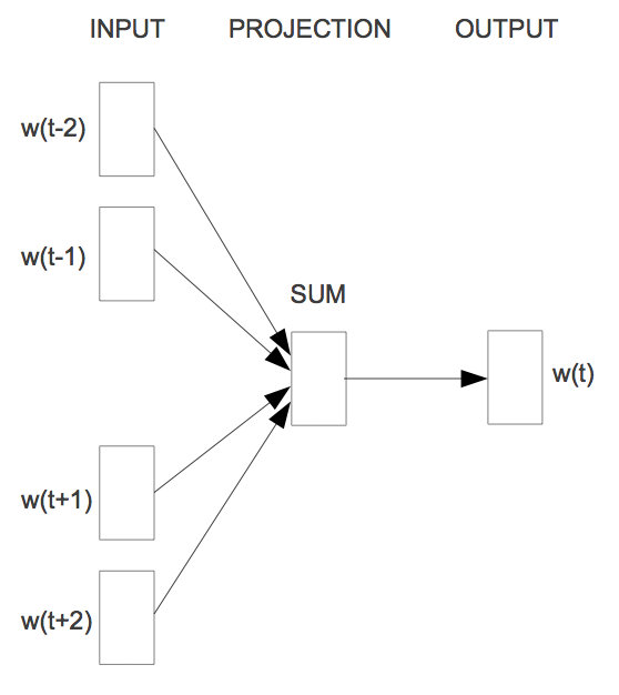
Continious Bag of Words (CBOW)
"Combination of context vectors predicts center word" $$L = \frac{1}{T}\sum\limits_{t=1}^T\ \text{log} \space p(w_t \: | \: w_{t-m} , \cdots , w_{t-1}, w_{t+1}, \cdots , w_{t+m})$$
SkipGram vs CBOW
- CBOW is faster during learning
- SkipGram is better for rare words
Word Vectors Evaluation
- Visual Exploration: whereby (a subsection of) the embeddings are displayed
- Intrinsic Evaluation: whereby the embeddings are used to perform a token-based task and the results are compared with a gold standard.
- Word Prediction: whereby we look into using a test corpus to evaluate the embeddings by defining a word prediction task.
- Extrinsic Evaluation: whereby a new model is learned (using the embeddings as inputs) to perform a complex task.
Visual Exploration
Use dimensionality reduction algorithms such as t-SNE and PCA to visualize (a subset) of the embedding space to project points to a 2-D or 3-D space.
- Pros:
- Can give you a sense of whether the model has correctly learned meaningful relations. Especially if you have a small number of pre-categorized words.
- Easy to explore the space
- Cons:
- Subjective: neighbourhoods may look good, but are they? There is no gold standard
- Works best for a small subset of the embedding space. But who decides which subset?
- resulting projection can be deceiving: what looks close in 3-D space can be far in 300-D space (and vice-versa).
Intrinsic Evaluation
Intrinsic evaluations are those where you can use embeddings to perform relatively simple, word-related tasks.
- Absolute intrinsic: you have a (human annotated) gold standard for a particular task and use the embeddings to make predictions.
- Comparative intrinsic: you use the embedding space to present predictions to humans, who then rate them. Mostly used when there is no gold standard available.
Tasks:
- Relatedness: How well do embeddings capture human-perceived word similarity? Datasets typically consist of triples: two words and a similarity score (e.g. between 0.0 and 1.0). Several available datasets, although interpretation of 'word similarity' can vary.
- Synonym detection: Can embeddings select a synonym for a given word and a set of options? Datasts are n-tuples where the first word is the input word and the other
n-1words are the options. Only one of the options is a synonym. - Analogy: Do embeddings encode relations between words? Datasets are 4-tuples: the first two words define the relation, the third word is the source of the query and the fourth word is the solution. Good embeddings should predict an embedding close to the solution word.
- Categorization: Can embeddings be clustered into hand-annotated categories? Datasets are word-category pairs. Standard clustering algorithms can then be used to generate k-clusters and the purity of the clusters can be computed.
- Selectional preference: Can embeddings predict whether a noun-verb pair is more likely to represent a verb-subject or a verb-object relation? E.g. people-eat is more likely to be found as a verb-subject.
Extrinsic Evaluation
In Extrinsic Evaluations, we have a more complex task we are interested in (e.g. text classification, text translation, image captioning), whereby we can use embeddings as a way to represent words (or tokens). Assuming we have:
- a model architecture and
- a corpus for training and evaluation (for which the embeddings provide adequate coverage),
we can then train the model using different embeddings and evaluate its overall performance. The idea is that better embeddings will make it easier for the model to learn the overall task.
Pretrained embeddings vs embedding learning
People have trained word2vec-like models on huge datasets:
On the other hand you have some text corpus for your specific task. Should you learn your own embeddings or use pretrained ones?
- Depends on your task
- simple task - use pretrained
- Depends on your dataset size
- not enough data - use pretrained
Anything2Vec
Ideas of word2vec can be transfered to any domain with proper data structure
Action2Vec
- Vocabulary: different tupes of user actions (clicks, cart actions, etc)
- Texts: sequence of actions
- Node2Vec
- Vocabulary: node ids
- Texts: sequence of node ids obtained via random walks
- URL2Vec
- Vocabulary: urls
- Texts: user sessions
References
- On word embeddings series (Sebastian Ruder) [blog]
- Distributed Representations of Words and Phrases and their Compositionality (Mikolov et al., 2013) [arxiv]
- Efficient Estimation of Word Representations in Vector Space (Mikolov et al., 2013) [arxiv]
- Distributed Representations of Sentences and Documents (Quoc Le et al., 2014) [arxiv]
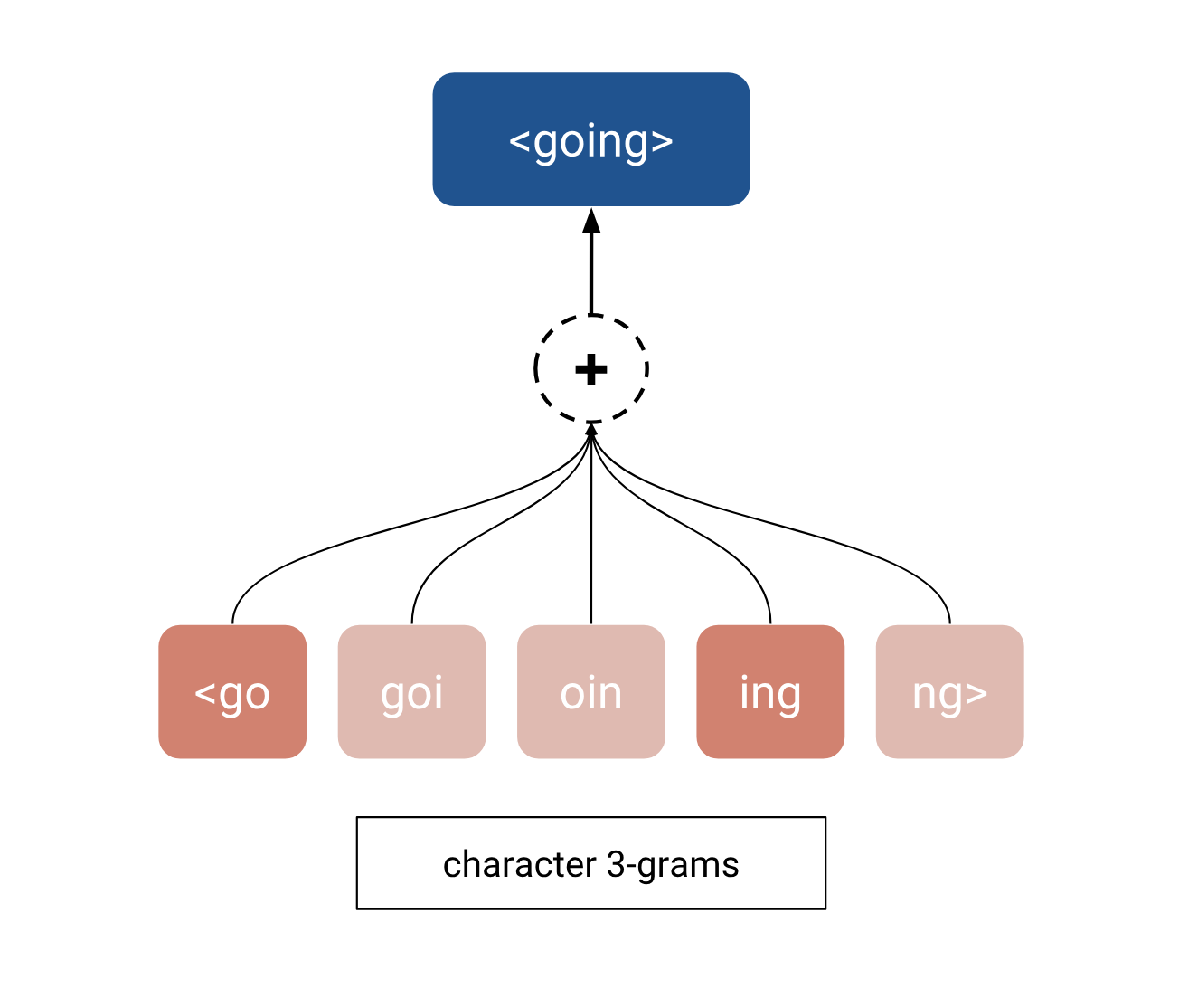
- Enriching word vectors with subword information (Bojanowski et al., 2016) [arxiv] (FastText)
- GloVe project page
- FastText project repo
Multidimentional scaling - intuinition
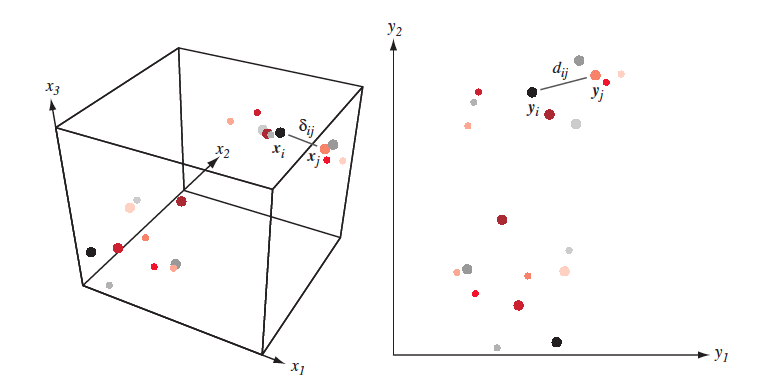
Find feature space with lesser dimentions s.t. distances in initial space are conserved in the new one. A bit more formally:
- Given $X = [x_1,\dots, x_n]\in \mathbb{R}^{N \times D}$ and/or $\delta_{ij}$ - proximity measure between $(x_i,x_j)$ in initial feature space.
- Find $Y = [y_1,\dots,y_n] \in \mathbb{R}^{N \times d}$ such that $\delta_{ij} \approx d(y_i, y_j) = \|y_i-y_j\|^2$
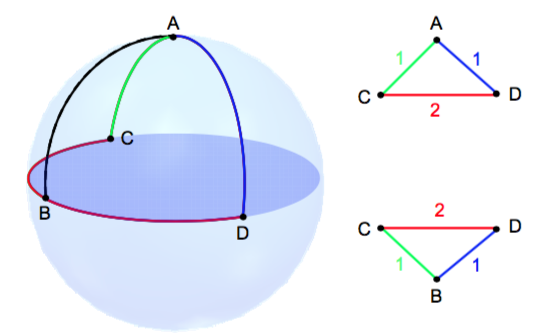
Multidimentional scaling
It is clear, that most of the times distances won't be conserved completely:
Multidimentional scaling approaches
- classical MDS (essentially PCA)
- metric MDS
- non-metric MDS
- But what if we want to conserve not the distances themselves, but the structure of inital dataset? Like neighbourhood of each point?
- Here comes t-SNE !!!
T-SNE
- t-SNE - is not multidimentional scaling, but the goal is somewhat similar
- There are going to be 3 types of similarities:
- Similarity between points in initial feature space
- Similarity between points in derived feature space
- Similarity between feature spaces!
T-SNE
- Similarity between points in initial feature space $\mathbb{R}^D$ $$ p(i, j) = \frac{p(i | j) + p(j | i)}{2N}, \quad p(j | i) = \frac{\exp(-\|\mathbf{x}_j-\mathbf{x}_i\|^2/{2 \sigma_i^2})}{\sum_{k \neq i}\exp(-\|\mathbf{x}_k-\mathbf{x}_i\|^2/{2 \sigma_i^2})} $$ $\sigma_i$ is set by user (implicitly)
- Similarity between points in derived feature space $\mathbb{R}^d, d << D$ $$ q(i, j) = \frac{g(|\mathbf{y}_i - \mathbf{y}_j|)}{\sum_{k \neq l} g(|\mathbf{y}_i - \mathbf{y}_j|)} $$ where $g(z) = \frac{1}{1 + z^2}$ - is student t-distribution with dof=$1$
- Similarity between feature spaces (Kullback–Leibler divergence) $$ J_{t-SNE}(y) = KL(P \| Q) = \sum_i \sum_j p(i, j) \log \frac{p(i, j)}{q(i, j)} \rightarrow \min\limits_{\mathbf{y}} $$
KL-Divergence
$$ KL(P \| Q) = \sum_z P(z) \log \frac{P(z)}{Q(z)} $$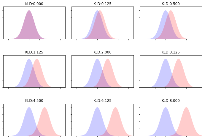
Optimization
- Optimize $J_{t-SNE}(y)$ with SGD
- Article
- Examples
- Demo and advises
- t-SNE is unstable
- Size of clusters means anything
- Distance means anything
- Random data can provide structure