Data Analysis

Andrey Shestakov (avshestakov@hse.ru)

Clustering¹

^{1. Some materials are taken from machine learning course of Victor Kitov}

Clustering¶

Aim of clustering¶

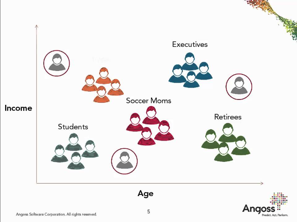
Clustering is partitioning of objects into groups so that:

inside groups objects are very similar
objects from different groups are dissimilar

Aim of clustering¶

Unsupervised learning
No definition of ''similar''
- different algorithms use different formalizations of similarity

Applications of clustering¶

data summarization
- feature vector is replaced by cluster number
feature extraction
- cluster number, cluster average target, distance to native cluster center / other clusters
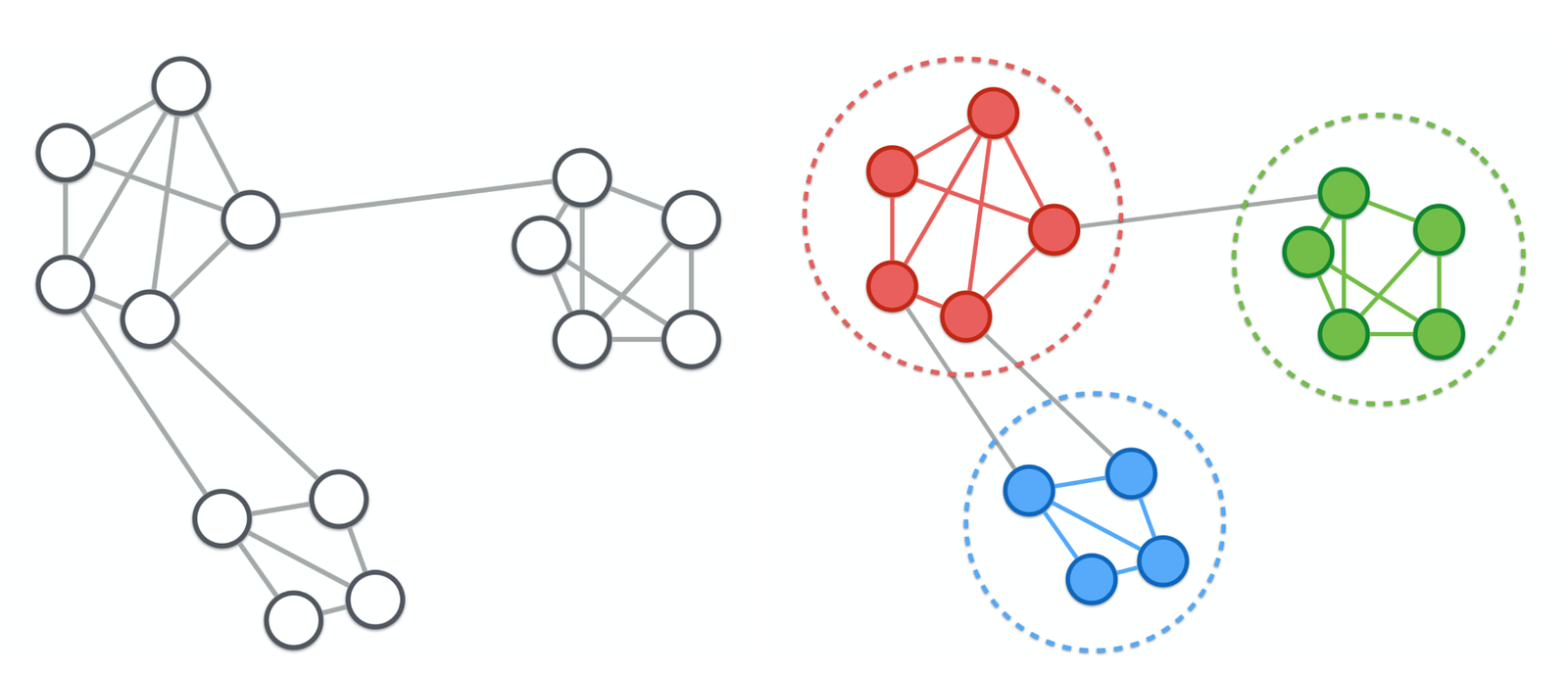
community detection in networks
- nodes - people, similarity - number of connections
outlier detection
- outliers do not belong any cluster

Groups of clustering methods¶

Prototype-based
- Replace cluster with ethalon object
Hierarchcal
- Build cluster hierarchy
Density-based
- Find dence groups of objects
Spectral
- Use spectral techniques
Grid-based
- Split feature space in grids and connect them
Probabilistic models
- Assume some mixture of probability distributions

Clustering algorithms comparison¶

We can compare clustering algorithms in terms of:

computational complexity
do they build flat or hierarchical clustering?
can the shape of clustering be arbitrary?
- if not is it symmetrical, can clusters be of different size?
can clusters vary in density of contained objects?
robustness to outliers

Prototype-based clustering¶

K-means¶

Prototype-based clustering¶

Clustering is flat (not hierarchical)
Number of clusters $K$ is specified in advance
Each object $x_{n}$ is associated with a cluster $z_{n}$
- $z_{n} \in \{1,\dots,K\}$
Each cluster $C_{k}$ is defined by its representative $\mu_{k}$, $k=1,2,...K.$
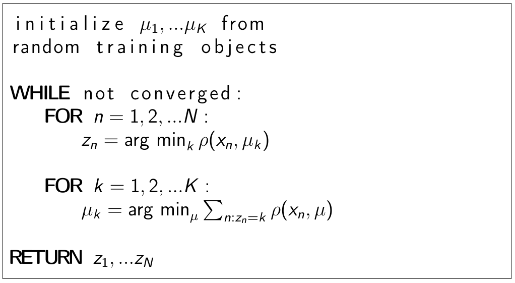
Criterion to find representatives $\mu_{1},...\mu_{K}$: $$ Q(z_{1},...z_{N})=\sum_{n=1}^{N}\min_{k}\rho(x_{n},\mu_{k})\to\min_{\mu_{1},...\mu_{K}} $$

Generic algorithm¶

Comments¶

different distance functions lead to different algorithms:
- $\rho(x,x')=\left\lVert x-x'\right\rVert _{2}^{2}$=> K-means
- $\rho(x,x')=\left\lVert x-x'\right\rVert _{1}$=> K-medians
$\mu_{k}$ may be arbitrary or constrained to be existing objects
$K$ - is set by user
- if chosen small=>distinct clusters will get merged
- better to take $K$ larger and then merge similar clusters.
Shape of clusters is defined by $\rho(\cdot,\cdot)$

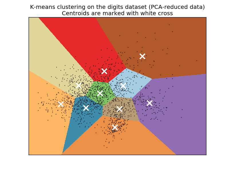
Example¶

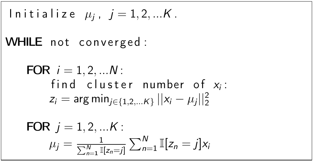
K-means algorithm¶

Suppose we want to cluster our data into $K$ clusters.
Cluster $i$ has a center $\mu_{i}$, i=1,2,...K.
Consider the task of minimizing $$ \sum_{n=1}^{N}\left\lVert x_{n}-\mu_{z_{n}}\right\rVert _{2}^{2}\to\min_{z_{1},...z_{N},\mu_{1},...\mu_{K}}\quad (1) $$ where $z_{i}\in\{1,2,...K\}$ is cluster assignment for $x_{i}$ and $\mu_{1},...\mu_{K}$ are cluster centers.
Direct optimization requires full search and is impractical.
K-means is a suboptimal algorithm for optimizing (1).

K-means algorithm¶

K-means properties¶

Convergence conditions
- maximum number of iterations reached
- cluster assignments $z_{1},...z_{N}$ stop to change (exact)
- $\{\mu_{i}\}_{i=1}^{K}$ stop changing significantly (approximate)
Initialization:
- typically $\{\mu_{i}\}_{i=1}^{K}$ are initialized to randomly chosen training objects

K-means properties¶

Optimality:
- criteria is non-convex
- solution depends on starting conditions
- may restart several times from different initializations and select solution giving minimal value of (1).
Complexity: $O(NDKI)$
- $K$ is the number of clusters
- $I$ is the number of iterations.
usually few iterations are enough for convergence.

Gotchas¶

K-means assumes that clusters are convex:
It always finds clusters even if none actually exist
- need to control cluster quality metrics

Main factors of solution¶

Initial position of centroids
Number of centroids

Number of centroids - K¶

Don't use vanilla k-means (X-means, ik-means)
Consider cluster quality measures
Use heuristics

Elbow method¶

Criterion of k-means $$ Q(C) = Q(z_{1},...z_{N}) = \sum_{n=1}^{N}\left\lVert x_{n}-\mu_{z_{n}}\right\rVert _{2}^{2}\to\min_{z_{1},...z_{N},\mu_{1},...\mu_{K}}\quad (1) $$
Lets take all possible values of $K$, and chose one that delivers minimum of $Q(C)$!

Won't work! Why?

In [3]:

from sklearn.datasets import make_blobs
from sklearn.cluster import KMeans

X, y = make_blobs(n_samples=500,
                  n_features=2,
                  centers=4,
                  cluster_std=1,
                  center_box=(-10.0, 10.0),
                  shuffle=True,
                  random_state=1) 


crit = []

for k in range(2, 8):
    kmeans = KMeans(n_clusters=k, random_state=1).fit(X)
    crit.append(np.sqrt(kmeans.inertia_))
    
def elbow_demo(k=2):
    
    X, y = make_blobs(n_samples=500,
                  n_features=2,
                  centers=4,
                  cluster_std=1,
                  center_box=(-10.0, 10.0),
                  shuffle=True,
                  random_state=1) 
    
    kmeans = KMeans(n_clusters=k, random_state=1).fit(X)
    
    fig, ax = plt.subplots(1,2)
    
    ax[0].scatter(X[:,0], X[:,1], c=kmeans.labels_)
    
    ax[0].scatter(kmeans.cluster_centers_[:, 0], kmeans.cluster_centers_[:, 1],
                  marker='o', c="white", alpha=1, s=200)
    
    ax[0].set_xlabel('$x_1$')
    ax[0].set_ylabel('$x_2$')

    for i, c in enumerate(kmeans.cluster_centers_):
        ax[0].scatter(c[0], c[1], marker='$%d$' % i, alpha=1, s=50)
        
    ax[1].plot(range(2,8), crit, marker='s')
    
    ax[1].set_xlabel('$k$')
    ax[1].set_ylabel('$Q^{(k)}(C)$')
    
    plt.show()

Elbow method¶

Choose $K$ after which $Q(C)$ stops decreasing rapidly
A bit more formally $$ D(k) = \frac{|Q^{(k)}(C) - Q^{(k+1)}(C)|}{|Q^{(k-1)}(C) - Q^{(k)}(C)|} \quad \text{" is small "} $$

In [4]:

plot = interact(elbow_demo, k=IntSlider(min=2,max=8,step=1,value=2))

Warning!¶

Heuristics are not dogma!
If at least some clusters are interpretable - this is good

Centroid initialization¶

Initiallize randombly
- Run multiple times and take result with smallest $Q(C)$
Use result of another clustering method as starting point
k-means++

K-means++¶

Choose 1st centroid randomly from initial objects
For each data point calculate its distance to closest centroid $d_{\min}(x_i) = \min_{\mu_j} \|x_i - \mu_j\|^2$
Take point as next centroid with probability $p(x_i) \propto d_{\min}(x_i)$

In [5]:

from sklearn.metrics import pairwise_distances

def demo_kmpp(iters=1):

    X, y = make_blobs(n_samples=550, cluster_std=1.5, n_features=2, centers=5, random_state=12345)

    X_grid1, X_grid2 = np.meshgrid(np.linspace(-12, 18, 500),
                                   np.linspace(-11, 8, 500))

    XX = np.c_[X_grid1.flatten(), X_grid2.flatten()]
    np.random.seed(1)
    centroids = np.empty((0, 2))

    for i in range(iters):
        if i == 0:
            d = np.ones_like(y, dtype=float)
        else:
            d = pairwise_distances(X, centroids, metric='euclidean').min(axis=1)
        weights = d/d.sum()

        centroid_idx = np.random.choice(X.shape[0], size=1, replace=False, p=weights)[0]
        centroids = np.r_[centroids, X[centroid_idx, np.newaxis]]

    d_grid = pairwise_distances(XX, centroids, metric='euclidean').min(axis=1)

    d_grid = d_grid.reshape(X_grid1.shape)
    d_grid = d_grid/d_grid.max()

    levels = np.linspace(0, 1, 100)

    plt.contourf(X_grid1, X_grid2, d_grid, cmap=plt.cm.Blues, alpha=0.7, levels=levels)
    plt.scatter(X[:, 0], X[:, 1], s=100)

    centers = centroids
    
    plt.scatter(centers[:, 0], centers[:, 1], marker='o',
                c="white", alpha=1, s=500, edgecolor='k')

    for i, c in enumerate(centers):
        plt.scatter(c[0], c[1], marker='$%d$' % (i+1), alpha=1,
                    s=100, edgecolor='k')

    plt.xlabel('$x_1$', fontsize=15)
    plt.ylabel('$x_2$', fontsize=15)

    plt.tight_layout()
    plt.axis('equal')
    plt.show()

In [6]:

interact(demo_kmpp, iters=IntSlider(min=1,max=6,step=1,value=1))

Out[6]:

<function __main__.demo_kmpp(iters=1)>

K-means¶

Not robust to outliers
- K-medians is a bit more robust
K-representatives may create singleton clusters in outliers if centroids get initialized with outlier
- better to init centroids with mean of $m$ randomly chosen objects
Constructs spherical clusters of similar radii
- Allows kernel version which can find non-convex clusters in original space

Hierarchical clustering¶

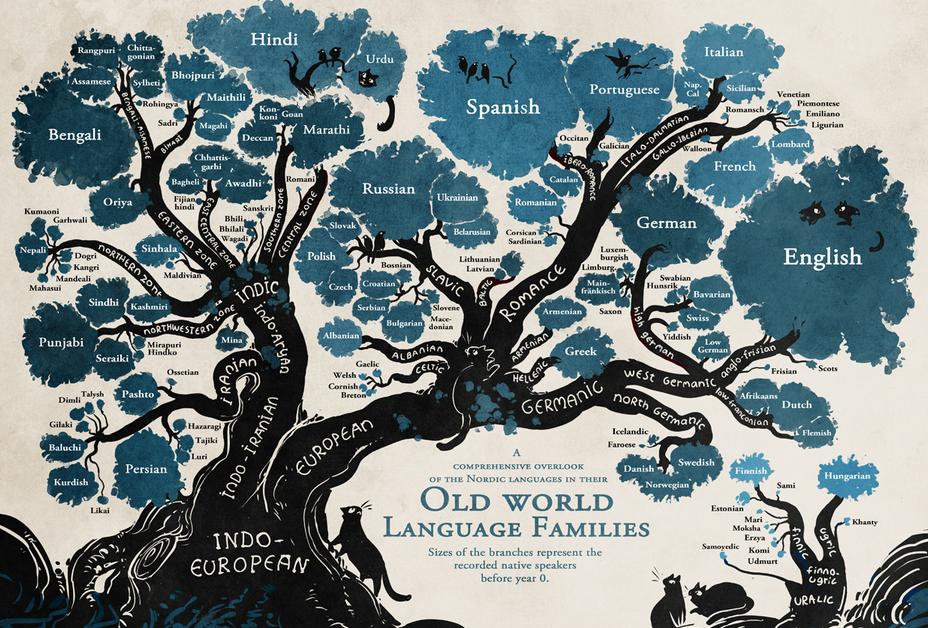
Insparation - Motivation¶

Number of clusters $K$ not known a priory.
Clustering is usually not flat, but hierarchical with different levels of granularity:
- sites in the Internet
- books in library
- animals in nature

Hierarchical clustering¶

Hierarchical clustering may be:

top-down
- divisive clustering
bottom-up
- aglomerative clustering

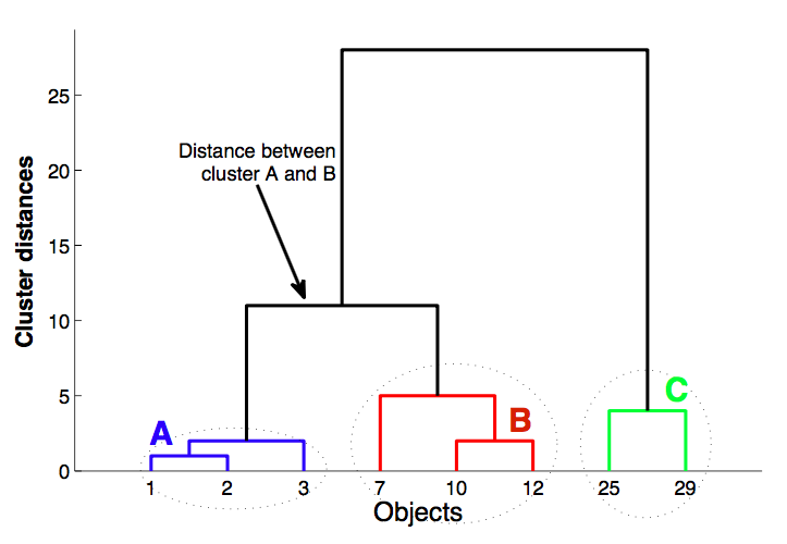
Aglomerative example¶

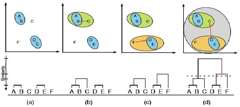
Dendrogram¶

Algorithm¶

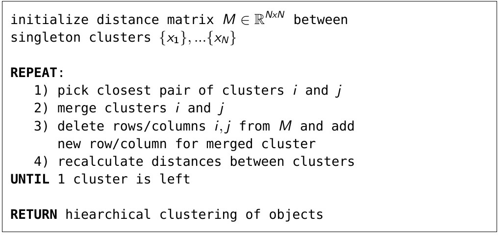
What is "closest pair of clusters"?
How do we recalculate distances between clusters?

Distance recalculation¶

Consider clusters $A=\{x_{i_{1}},x_{i_{2}},...\}$ and $B=\{x_{j_{1}},x_{j_{2}},...\}$.
We can define the following natural ways to recalculate distances
- nearest neighbour (or single link) $$ \rho(A,B)=\min_{a\in A,b\in B}\rho(a,b) $$
- furthest neighbour (or complete link) $$ \rho(A,B)=\max_{a\in A,b\in B}\rho(a,b) $$
- group average link $$ \rho(A,B)=\frac{1}{N_AN_B}\sum\limits_{a\in A,b\in B}\rho(a,b) $$
- closest centroid (or centroid-link) $$ \rho(A,B)=\rho(\mu_{A},\mu_{B}) $$ where $\mu_{U}=\frac{1}{|U|}\sum_{x\in U}x$ or $m_{U}=median_{x\in U}\{x\}$

Lance–Williams formula¶

$$ \rho(C_i \cup C_j, C_k) = a_i \cdot \rho(C_i, C_k) + a_j \cdot \rho(C_j, C_k) + b \cdot \rho(C_i, C_j) + c \cdot |\rho(C_i, C_k) - \rho(C_j, C_k)|$$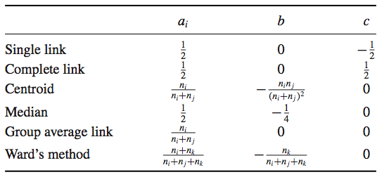

Heuristics for dendrogram quality¶

cophenetic distance between objects $x_i$ и $x_j$ - height of dendrogram at which whose two objects have merged

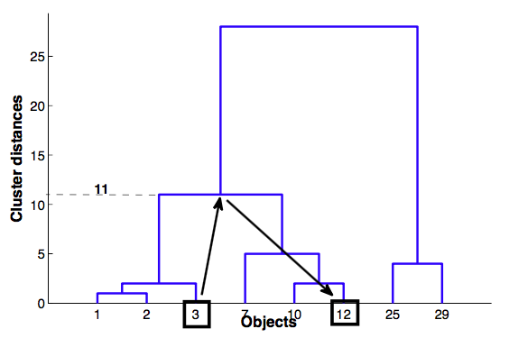
Cophenetic correlation¶

Cophenetic correlation — correlation between Cophenetic distance and simple distance between objects

$$ \text{cophCorr} = \frac{\sum\limits_{i < j}(d(x_i, x_j) - \bar{d})(coph(x_i, x_j) - \bar{coph})}{\sqrt{\sum\limits_{i < j}(d(x_i, x_j) - \bar{d})^2 \cdot \sum\limits_{i < j}(coph(x_i, x_j) - \bar{coph})^2}} $$

If dendrogram is good, correlation should be high

In [7]:

# А теперь сделаем это с питоном
from scipy.cluster.hierarchy import dendrogram, linkage 
from scipy.cluster.hierarchy import fcluster, cophenet

from scipy.spatial.distance import pdist

def coph_demo(link='single', metric='euclidean', k=2):
    
    X, y = make_blobs(n_samples=500,
                  n_features=2,
                  centers=4,
                  cluster_std=1,
                  center_box=(-10.0, 10.0),
                  shuffle=True,
                  random_state=1) 
    
    d = pdist(X, metric=metric)
    
    Z = linkage(X, method=link, metric=metric)
    labels = fcluster(Z,  k, criterion='maxclust')
    
    fig, ax = plt.subplots(1,2)
    
    ax[0].scatter(X[:,0], X[:,1], c=labels)
        
    ax[0].set_xlabel('$x_1$')
    ax[0].set_ylabel('$x_2$')
        
    dend = dendrogram(Z, ax=ax[1], truncate_mode='lastp')   
    coph_corr, coph_dist = cophenet(Z, d)
    
    ax[1].set_title('cophCorr = %.3f' % coph_corr)
    
    plt.show()

In [8]:

interact(coph_demo, k=IntSlider(min=2, max=10, step=1, value=2), link=['complete', 'single', 'average', 'centroid'], metric=['euclidean', 'cityblock'])

Out[8]:

<function __main__.coph_demo(link='single', metric='euclidean', k=2)>

Comments¶

Results in full hierarchy of objects
Various ways to calculate distances
Nice visualization
Needs a lot of resources

Density-based methods¶

DBScan¶

Goal¶

Identify clusters as groups of densly connected points, separated by sparse areas

Idea¶

Identify 2 parameters
- $\epsilon$ - radius of neighbourhood of each point. $N_\epsilon(p)$ - neighbourhood of point $p$
- min_pts - minimal number of points inside neighbourhood
To start a cluster from point there should be at least min_pts points in $N_\epsilon$
If this conditions is satisfied - spread cluster and check all points neighbours by the same crierion

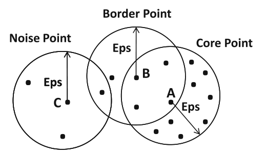
Types of points¶

Core point: point having $\ge \texttt{min_pts}$ points in its $\varepsilon$ neighbourhood
Border point: not core point, having at least 1 core point in its $\varepsilon$ neighbourhood
Noise point: neither a core point nor a border point

Demo¶

Click

DBSCAN¶

{C}
1.function dbscan(X, eps, min_pts):
2.  initialize NV = X # not visited objects 
3.  for x in NV:
4.      remove(NV, x) # mark as visited
5.      nbr = neighbours(x, eps) # set of neighbours
6.      if nbr.size < min_pts:
7.          mark_as_noise(x)
8.      else:
9.          C = new_cluster() 
10.         expand_cluster(x, nbr, C, eps, min_pts, NV)
11.         yield C

expand_cluster¶

{C}
1. function expand_cluster(x, nbr, C, eps, min_pts, NV):
2.  add(x, C)
3.  for x1 in nbr:
4.      if x1 in NV: # object not visited
5.          remove(NV, x1) # mark as visited
6.          nbr1 = neighbours(x1, eps)
7.          if nbr1.size >= min_pts:
8.              # join sets of neighbours
9.              merge(nbr, nbr_1) 
10.     if x1 not in any cluster:
11.         add(x1, C)

In [10]:

interact(dbscan_demo, eps=FloatSlider(min=0.1, max=10, step=0.05, value=1), min_pts=IntSlider(min=2, max=15, step=1, value=5))

Out[10]:

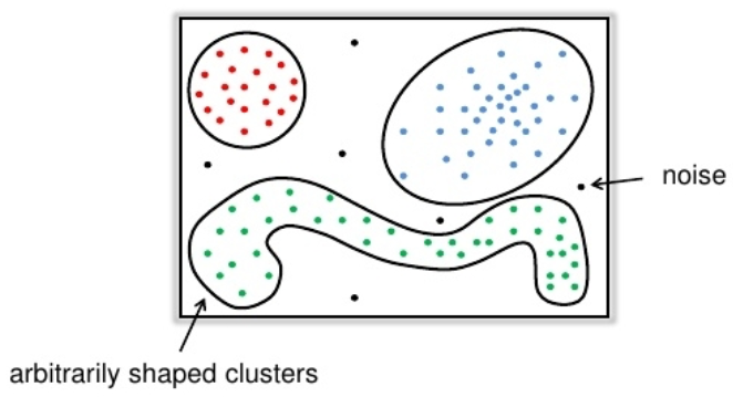
<function __main__.dbscan_demo(eps=1, min_pts=5)>

Recap¶

Do not indicate number of clusters
Arbitrary shapes of clusters
Identifies outliers
Problems with varying density

Failure for varying density¶

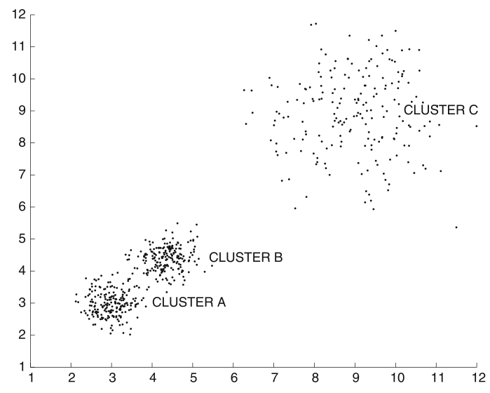
Large min_pts: cluster C is missed
Small min_pts: clusters A and B get merged

Cluster Validity and Quality Measures¶

General approaches¶

Evaluate using "ground-truth" clustering (Quality Measure)
- invariant to cluster naming
Unsupervised criterion (Cluster Validity)
- based on intuition:
  - objects from same cluster should be similar
  - objects from different clusters should be different

Based on ground-truth¶

Rand Index¶

$$ \text{Rand}(\hat{\pi},\pi^*) = \frac{a + d}{a + b + c + d} \text{,}$$

where

$a$ - number of pairs that are grouped both in $\hat{\pi}$ and
$d$ - number of pairs that are separated both in $\hat{\pi}$ and $\pi^*$ $\pi^*$,
$b$ ($c$) - number of pairs that are separated both in $\hat{\pi}$ ($\pi^*$), but grouped in $\pi^*$ ($\hat{\pi}$)

Rand Index¶

$$ \text{Rand}(\hat{\pi},\pi^*) = \frac{tp + tn}{tp + fp + fn + tn} \text{,}$$

where

$tp$ - number of pairs that are grouped both in $\hat{\pi}$ and
$tn$ - number of pairs that are separated both in $\hat{\pi}$ and $\pi^*$ $\pi^*$,
$fp$ ($fn$) - number of pairs that are separated both in $\hat{\pi}$ ($\pi^*$), but grouped in $\pi^*$ ($\hat{\pi}$)

Adjusted Rand Index

$$\text{ARI}(\hat{\pi},\pi^*) = \frac{\text{Rand}(\hat{\pi},\pi^*) - \text{Expected}}{\text{Max} - \text{Expected}}$$

Precision, Recall, F-measure¶

$\text{Precision}(\hat{\pi},\pi^*) = \frac{tp}{tp+fn}$
$\text{Recall}(\hat{\pi},\pi^*) = \frac{tp}{tp+fp}$
$\text{F-measure}(\hat{\pi},\pi^*) = \frac{2\cdot Precision \cdot Recall}{Precision + Recall}$

Cluster validity¶

Intuition
- objects from same cluster should be similar
- objects from different clusters should be different

Silhouette¶

For each object $x_{i}$ define:

$s_{i}$-mean distance to objects in the same cluster
$d_{i}$-mean distance to objects in the next nearest cluster Silhouette coefficient for $x_{i}$: $$ Silhouette_{i}=\frac{d_{i}-s_{i}}{\max\{d_{i},s_{i}\}} $$

Silhouette coefficient for $x_{1},...x_{N}$: $$ Silhouette=\frac{1}{N}\sum_{i=1}^{N}\frac{d_{i}-s_{i}}{\max\{d_{i},s_{i}\}} $$

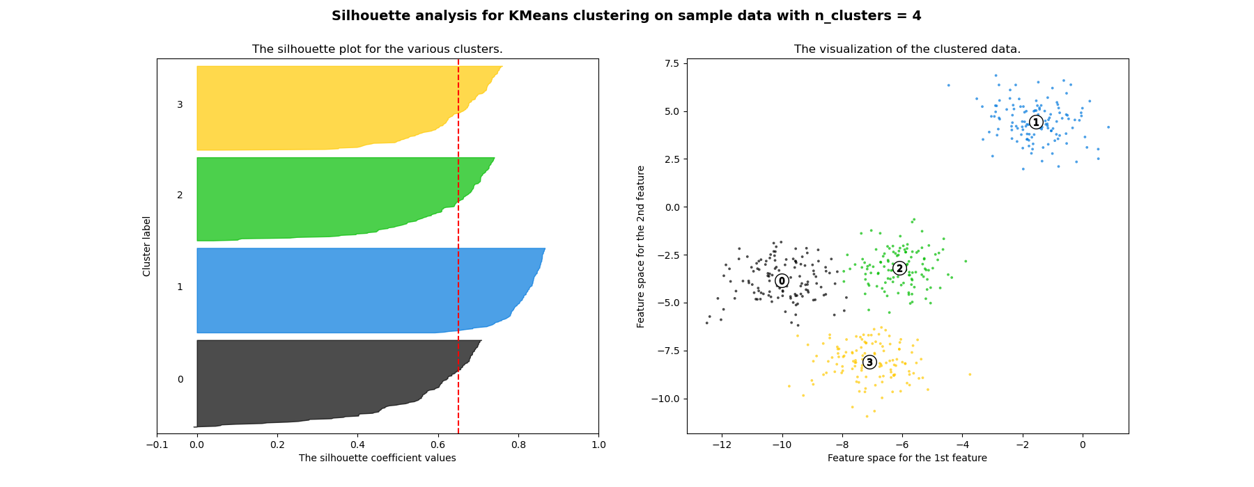
Discussion¶

Advantages
- The score is bounded between -1 for incorrect clustering and +1 for highly dense clustering.
- Scores around zero indicate overlapping clusters.
- The score is higher when clusters are dense and well separated.
Disadvantages
- complexity $O(N^{2}D)$
- favours convex clusters

FYI¶

What else?¶

Mixture Models (maybe next)
Spectral clustering
Community Detection
Consensus clustering!

Data Analysis

Andrey Shestakov (avshestakov@hse.ru)

Clustering1

Clustering¶

Aim of clustering¶

Aim of clustering¶

Applications of clustering¶

Groups of clustering methods¶

Clustering algorithms comparison¶

Prototype-based clustering¶

K-means¶

Prototype-based clustering¶

Generic algorithm¶

Comments¶

Example¶

K-means algorithm¶

K-means algorithm¶

K-means properties¶

K-means properties¶

Gotchas¶

Main factors of solution¶

Number of centroids - K¶

Elbow method¶

Elbow method¶

Warning!¶

Centroid initialization¶

K-means++¶

K-means¶

Hierarchical clustering¶

Insparation - Motivation¶

Insparation - Motivation¶

Hierarchical clustering¶

Aglomerative example¶

Dendrogram¶

Algorithm¶

Distance recalculation¶

Lance–Williams formula¶

Heuristics for dendrogram quality¶

Cophenetic correlation¶

Comments¶

Density-based methods¶

DBScan¶

Goal¶

Idea¶

Types of points¶

Demo¶

DBSCAN¶

expand_cluster¶

Recap¶

Failure for varying density¶

Cluster Validity and Quality Measures¶

General approaches¶

Based on ground-truth¶

Rand Index¶

Rand Index¶

Precision, Recall, F-measure¶

Cluster validity¶

Silhouette¶

Discussion¶

FYI¶

What else?¶

Clustering¹